
Abstract
In this paper, we formulate the problem of elastodynamic transformation cloaking for Kirchoff–Love plates and elastic plates with both in-plane and out-of-plane displacements. A cloaking transformation maps the boundary-value problem of an isotropic and homogeneous elastic plate (virtual problem) to that of an anisotropic and inhomogeneous elastic plate with a hole surrounded by a cloak that is to be designed (physical problem). For Kirchoff–Love plates, the governing equation of the virtual plate is transformed to that of the physical plate up to an unknown scalar field. In doing so, one finds the initial stress and the initial tangential body force for the physical plate, along with a set of constraints that we call the cloaking compatibility equations. It is noted that the cloaking map needs to satisfy certain boundary and continuity conditions on the outer boundary of the cloak and the surface of the hole. In particular, the cloaking map needs to fix the outer boundary of the cloak up to the third order. Assuming a generic radial cloaking map, we show that cloaking a circular hole in Kirchoff–Love plates is not possible; the cloaking compatibility equations and the boundary conditions are the obstruction to cloaking. Next, relaxing the pure bending assumption, the transformation cloaking problem of an elastic plate in the presence of in-plane and out-of-plane displacements is formulated. In this case, there are two sets of governing equations that need to be simultaneously transformed under a cloaking map. We show that cloaking a circular hole is not possible for a general radial cloaking map; similar to Kirchoff–Love plates, the cloaking compatibility equations and the boundary conditions obstruct transformation cloaking. Our analysis suggests that the path forward for cloaking flexural waves in plates is approximate cloaking formulated as an optimal design problem.

We’re sorry, something doesn't seem to be working properly.
Please try refreshing the page. If that doesn't work, please contact support so we can address the problem.
Notes
They, however, do not provide a clear mathematical reasoning as to why Colquitt et al. (2014)’s formulation is incorrect.
One should note that in formulating a cloaking problem one can either transform the action and then use Hamilton’s principle for the transformed action or simply transform the Euler–Lagrange equations if they are derived covariantly, i.e., the tensorial form of all quantities are retained and there is a clear distinction between the referential and spatial coordinates.
Note the typo in the expression for \(S_{I}\) in their Eq. (14).
A linear connection is said to be compatible with a metric \(\bar{{\mathbf {G}}}\) on the manifold provided that

where \(\left\langle \left\langle .,. \right\rangle \right\rangle _{\bar{{\mathbf {G}}}}\) is the inner product induced by the metric \(\bar{{\mathbf {G}}}\). It is straightforward to show that \({\bar{\nabla }}\) is compatible with \(\bar{{\mathbf {G}}}\) if and only if \({\bar{\nabla }}\bar{{\mathbf {G}}}={\mathbf {0}}\), or, in components
$$\begin{aligned} {\bar{G}}_{AB|C}=\frac{\partial {\bar{G}}_{AB}}{\partial X^C}-{\bar{\Gamma }}^S{}_{CA}{\bar{G}}_{SB}-{\bar{\Gamma }}^S{}_{CB}{\bar{G}}_{AS}=0. \end{aligned}$$On any Riemannian manifold \(({\mathcal {B}},\bar{{\mathbf {G}}})\) the Levi–Civita connection is the unique linear connection \({\bar{\nabla }}^{\bar{{\mathbf {G}}}}\) that is compatible with \(\bar{{\mathbf {G}}}\) and is symmetric (torsion-free). Note that the metric compatibility of \({\bar{\nabla }}\) (see (2.4)) and the fact that \(\bar{{\mathbf {G}}}(\bar{{\mathbf {N}}},\bar{{\mathbf {Y}}})=0\) are used in deriving the second equality in (2.5).
Note that for \(X\in {\mathcal {H}}\), the metric (2.13) has the following representation
$$\begin{aligned} \bar{{\mathbf {G}}}(X)=\begin{bmatrix} {\bar{G}}_{11}(X) &{} {\bar{G}}_{12}(X) &{} 0 \\ {\bar{G}}_{12}(X) &{} {\bar{G}}_{22}(X) &{} 0 \\ 0 &{} 0 &{} 1 \end{bmatrix}, \end{aligned}$$Note that the first and the second fundamental forms of \({\mathcal {H}}\) can be expressed in terms of the metric of the embedding space \({\mathcal {B}}\) given by \(\left[ \begin{array}{cc}{\bar{G}}_{11}&{}{\bar{G}}_{12}\\ {\bar{G}}_{12}&{}{\bar{G}}_{22}\end{array} \right] (X)\), \(X\in {\mathcal {B}}\), which in turn, fully characterizes the geometry of \({\mathcal {H}}\).
See (Simo et al. 1988) for another equivalent way of characterizing the configuration space of a plate.
Note that in coordinates \((x^1,x^2,x^3)\), for which \(x^3\) is the outward normal direction, the second fundamental form of the deformed shell is expressed as
$$\begin{aligned} \theta _{ab}=-\frac{1}{2}\frac{\partial {\bar{g}}_{ab}}{\partial x^3}\Big |_{\varphi ({\mathcal {H}})}(x), \quad a,b=1,2,\quad \forall x\in \varphi ({\mathcal {H}}). \end{aligned}$$See (Ericksen and Truesdell 1957, P.313) for a discussion on the compatibility equations of a Cosserat shell with deformable directors.
Note that \(T_{(X,t)}\varphi \) (cf. (2.25)) is injective, and hence, the local extension vector field always exists, unless \({\mathbf {V}}\) is purely tangential, i.e., \({{\mathbf {V}}}^\perp ={\mathbf {0}}\). In this case, however, one does not need a local extension to compute the acceleration unambiguously as \({\mathbf {V}}={\mathbf {V}}^\top \), and hence, \({\mathbf {A}}(X,t)={\bar{\nabla }}^{\bar{{\mathbf {g}}}}_{{\mathbf {V}}}{\mathbf {V}}={\bar{\nabla }}^{\bar{{\mathbf {g}}}}_{{{\mathbf {V}}}^\top }{\mathbf {V}}^\top \).
Let \({\mathbf {W}}\in {\mathcal {X}}(\varphi _t({\mathcal {H}}))\) be an arbitrary vector field defined in a neighborhood containing \((X_o,t_o)\). Thus, \(\bar{{\mathbf {g}}}(\varvec{{\mathcal {V}}}^\perp ,{\mathbf {W}})=0\), and from (2.4), \(\bar{{\mathbf {g}}}({\bar{\nabla }}^{\bar{{\mathbf {g}}}}_{\varvec{{\mathcal {V}}}}{\varvec{{\mathcal {V}}}}^\perp ,{\mathbf {W}})=-\bar{{\mathbf {g}}}({\varvec{{\mathcal {V}}}}^\perp ,{\bar{\nabla }}^{\bar{{\mathbf {g}}}}_{\varvec{{\mathcal {V}}}}{\mathbf {W}})\). Note that
$$\begin{aligned} \begin{aligned} {\bar{\nabla }}^{\bar{{\mathbf {g}}}}_{\varvec{{\mathcal {V}}}}{\mathbf {W}}&=[\varvec{{\mathcal {V}}},{\mathbf {W}}]+{\bar{\nabla }}^{\bar{{\mathbf {g}}}} _{{\mathbf {W}}}\varvec{{\mathcal {V}}}=[\varvec{{\mathcal {V}}},{\mathbf {W}}] +{\bar{\nabla }}^{\bar{{\mathbf {g}}}}_{{\mathbf {W}}}{\varvec{{\mathcal {V}}}}^\top +{\bar{\nabla }}^{\bar{{\mathbf {g}}}}_{{\mathbf {W}}}{\varvec{{\mathcal {V}}}}^\perp \\&=[\varvec{{\mathcal {V}}},{\mathbf {W}}]+{\nabla }^{{\mathbf {g}}}_{{\mathbf {W}}}{{\varvec{{\mathcal {V}}}}}^\top +\varvec{\theta }({{\varvec{{\mathcal {V}}}}}^\top ,{\mathbf {W}}){\mathbf {n}}+(d{\mathcal {V}}^\perp \cdot {\mathbf {W}}){\mathbf {n}}+{\mathcal {V}}^\perp {{\bar{\nabla }}}^{\bar{{\mathbf {g}}}}_{{\mathbf {W}}}{\mathbf {n}}. \end{aligned} \end{aligned}$$Thus, noting that \([\varvec{{\mathcal {V}}},{\mathbf {W}}]\), \({\nabla }^{{\mathbf {g}}}_{{\mathbf {W}}}{{\varvec{{\mathcal {V}}}}}^\top \), \({\mathcal {V}}^\perp {{\bar{\nabla }}}^{\bar{{\mathbf {g}}}}_{{\mathbf {W}}}{\mathbf {n}}\in {\mathcal {X}}(\varphi _t({\mathcal {H}}))\) one concludes that \(\bar{{\mathbf {g}}}(\varvec{{\mathcal {V}}}^\perp ,{\bar{\nabla }}^{\bar{{\mathbf {g}}}}_{\varvec{{\mathcal {V}}}}{\mathbf {W}})={\mathcal {V}}^\perp \varvec{\theta }({{\varvec{{\mathcal {V}}}}}^\top ,{\mathbf {W}})+{\mathcal {V}}^\perp (d{\mathcal {V}}^\perp \cdot {\mathbf {W}})\), which by arbitrariness of \({\mathbf {W}}\) together with \(\bar{{\mathbf {g}}}({\bar{\nabla }}^{\bar{{\mathbf {g}}}}_{\varvec{{\mathcal {V}}}}{\varvec{{\mathcal {V}}}}^\perp ,{\mathbf {W}})=-\bar{{\mathbf {g}}}({\varvec{{\mathcal {V}}}}^\perp ,{\bar{\nabla }}^{\bar{{\mathbf {g}}}}_{\varvec{{\mathcal {V}}}}{\mathbf {W}})\) implies (2.34).
Consider a surface embedded in the ambient space such that the embedding is given as \(\varphi : {\mathcal {H}}\rightarrow {\mathcal {S}}\), where for the sake of simplicity one can assume that \({\mathcal {S}}={\mathbb {R}}^3\). The fundamental theorem of surface theory proved by Bonnet (1867) implies that the surface geometry (up to rigid body motions) is completely characterized by the induced first and second fundamental forms \({\mathbf {C}}\) and \({\varvec{\Theta }}\). Therefore, the surface energy density must depend on \({\mathbf {C}}\) and \(\varvec{\Theta }\).
\(D_{\varphi _{\epsilon }(X,t)}\) denotes the covariant derivative along the curve \(\varphi _{\epsilon }(X,t)\).
Note that (3.31) is equivalent to \(\sigma ^{ab}\) and \({\mathcal {M}}^{ab}\) being symmetric.
Note that in the local coordinate chart \(\{x^1,x^2,x^3\}\), for which \(x^3\) is the outward normal direction
$$\begin{aligned} \theta _{ab}=-\frac{1}{2}\frac{\partial {\bar{g}}_{ab}}{\partial x^3}\Big |_{\varphi ({\mathcal {H}})},\quad a,b=1,2. \end{aligned}$$Thus,
$$\begin{aligned} (\psi _{s*}\theta )_{ a' b'}= & {} -\frac{1}{2}\frac{\partial \left( (T\psi _s^{-1})^a{}_{ a'}(T\psi _s^{-1})^b{}_{ b'}{\bar{g}}_{ab}\right) }{\partial x^3}=(T\psi _s^{-1})^a{}_{ a'}(T\psi _s^{-1})^b{}_{ b'}\left( -\frac{1}{2}\frac{\partial {\bar{g}}_{ab}}{\partial x^3}\right) \\= & {} (T\psi _s^{-1})^a{}_{ a'}(T\psi _s^{-1})^b{}_{ b'}\theta _{ab},\quad a',b'=1,2. \end{aligned}$$Note also that \((T\psi ^{-1}_{s})^{a}{}_{a'}=-\delta ^b{}_{a'}\delta ^a{}_{b'}(T\psi _{s})^{b'}{}_b\).
Note that \({\dot{\varrho }}=\frac{\partial \varrho }{\partial t}+\nabla \varrho \cdot {\mathbf {v}}\).
Note that we do not explicitly specify the source of the initial stress or couple-stress. If the initial stress and couple-stress are due to elastic deformations, and the body has an energy function W with respect to its stress-free configuration, then one may express \(\mathring{{\mathbf {P}}}\) and \(\mathring{{{{\mathbf {\mathsf{{M}}}}}}}\) as
$$\begin{aligned} \mathring{{\mathbf {P}}}=2\mathring{{\mathbf {F}}}\frac{\partial W}{\partial {\mathbf {C}}}\Big |_{\mathring{{\mathbf {F}}}}, \quad \mathring{{{{\mathbf {\mathsf{{M}}}}}}}=\mathring{{\mathbf {F}}} \frac{\partial W}{\partial {\varvec{\Theta }}}\Big |_{\mathring{{\mathbf {F}}}}. \end{aligned}$$Note that the variation of the normal vector \(\delta \varvec{{\mathcal {N}}}\) is purely tangential, and hence, so is the term \({\bar{{\mathbf {g}}}}(\mathring{\varvec{{\mathfrak {B}}}},\varvec{{\mathcal {N}}})\delta \varvec{{\mathcal {N}}}\) in (3.76). In (3.77), with an abuse of notation we only consider the term in the normal direction.
Note that for cloaking applications considered in this paper \({\tilde{\varphi }}_t=id\), i.e., the identity map, and \(\varphi _t\) is time-independent but is not necessarily the identity map as we assume a time-independent pre-stress distribution for the cloak.
The Piola transformation of a vector (field) \({\mathbf {w}}\in T_{\varphi (X)}{\mathcal {S}}\) is a vector \({\mathbf {W}}\in T_X{\mathcal {B}}\) given by \({\mathbf {W}}=J\varphi ^*{\mathbf {w}}=J{\mathbf {F}}^{-1}{\mathbf {w}}\). In coordinates, one has \(W^A=J(F^{-1})^A{}_bw^b\), where \(J=\sqrt{\frac{\det {\mathbf {g}}}{\det {\mathbf {G}}}}\det {\mathbf {F}}\) is the Jacobian of \(\varphi \) with \({\mathbf {G}}\) and \({\mathbf {g}}\) the Riemannian metrics of \({\mathcal {B}}\) and \({\mathcal {S}}\), respectively. Note that a Piola transformation can be performed on any index of a given tensor. One can show that \({\text {Div}}{\mathbf {W}}=J({\text {div}}{\mathbf {w}})\circ \varphi \), which in coordinates is written as \(W^A{}_{|A}=Jw^a{}_{|a}\). This is also known as the Piola identity. Another way of writing the Piola identity is in terms of the unit normal vectors of a surface in \({\mathcal {B}}\) and its corresponding surface in \({\mathcal {S}}\), along with the area elements. It is written as \(\hat{{\mathbf {n}}}da=J{\mathbf {F}}^{-\star }\hat{{\mathbf {N}}}dA\), or in components, one writes \(n_ada=J(F^{-1})^A{}_aN_AdA\). In the literature of continuum mechanics, this is known as Nanson’s formula.
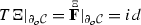
Note that for both plates we may use two global collinear Cartesian coordinates \(\{z^1,z^2,z^3\}\) and \(\{{\tilde{z}}^1,{\tilde{z}}^2,{\tilde{z}}^3\}\) such that \(z^3\) and \({\tilde{z}}^3\) are the outward normal directions to the physical and virtual plates, respectively. Therefore, \(\{z^1,z^2\}\) and \(\{{\tilde{z}}^1,{\tilde{z}}^2\}\) are two global collinear Cartesian coordinates for \(\varphi ({\mathcal {H}})\) and \({\tilde{\varphi }}(\tilde{{\mathcal {H}}})\), respectively, where \(\Xi :{\mathcal {H}}\rightarrow \tilde{{\mathcal {H}}}\), \(\varphi :{\mathcal {H}}\rightarrow \varphi ({\mathcal {H}})\), \({\tilde{\varphi }}:\tilde{{\mathcal {H}}}\rightarrow {\tilde{\varphi }}(\tilde{{\mathcal {H}}})\), and \(\xi :\varphi ({\mathcal {H}})\rightarrow {\tilde{\varphi }}(\tilde{{\mathcal {H}}})\), and \({{{\mathbf {\mathsf{{s}}}}}}\) is defined as
$$\begin{aligned} {\mathsf {s}}^{{\tilde{a}}}{}_a(x)=\frac{\partial {\tilde{x}}^{{\tilde{a}}}}{\partial {\tilde{z}}^{{\tilde{i}}}}({\tilde{x}}) \frac{\partial z^i}{\partial x^a}(x) \delta ^{{\tilde{i}}}_i,~~~a,{\tilde{a}},i,{\tilde{i}}=1,2 , \end{aligned}$$where \(\{x^a\}\) and \(\{{\tilde{x}}^{{{\tilde{a}}}}\}\) are local coordinate charts for \(\varphi ({\mathcal {H}})\) and \({\tilde{\varphi }}(\tilde{{\mathcal {H}}})\), respectively.
See Remark. 3.1 for a discussion on how the boundary surface traction, boundary shear force, and boundary moment as well as their corresponding Dirichlet boundary conditions are prescribed in the boundary-value problem.
Note that introducing the scalar field \(k=k(X)\) provides an extra degree of freedom in the cloaking problem. It has to be positive because \(\rho =k{\tilde{\rho }}\circ \Xi \).
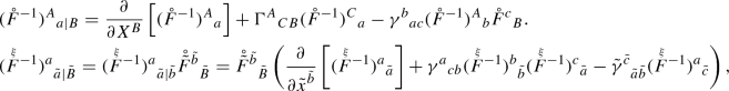
The covariant derivative of a two-point tensor \({\mathbf {T}}\) is given by
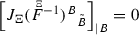
$$\begin{aligned} \begin{aligned} T^{AB\cdots F}{}_{G\cdots Q}{}^{ab\cdots f}{}_{g\cdots q|K}&=\frac{\partial }{\partial X^K}T^{AB\cdots F}{}_{G\cdots Q}{}^{ab\cdots f}{}_{g\cdots q}\\&\quad +T^{RB\cdots F}{}_{G\cdots Q}{}^{ab\cdots f}{}_{g\cdots q}\Gamma ^A{}_{RK}+\mathrm {(all\,\,upper\,\, referential\,\, indices)}\\&\quad -T^{AB\cdots F}{}_{R\cdots Q}{}^{ab\cdots f}{}_{g\cdots q}\Gamma ^R{}_{GK}-\mathrm {(all\,\,lower\,\, referential\,\, indices)}\\&\quad +T^{AB\cdots F}{}_{G\cdots Q}{}^{lb\cdots f}{}_{g\cdots q}\gamma ^a{}_{lr}F^r{}_K+\mathrm {(all\,\,upper\,\, spatial\,\, indices)}\\&\quad -T^{AB\cdots F}{}_{G\cdots Q}{}^{ab\cdots f}{}_{l\cdots q}\gamma ^l{}_{gr}F^r{}_K-\mathrm {(all\,\,lower\,\, spatial\,\, indices)}. \end{aligned} \end{aligned}$$Pomot et al. (2019) used a linear cloaking transformation, which has a covarianlty constant tangent map. However, a linear cloaking map does not satisfy the required traction boundary condition on \(\partial _o{\mathcal {C}}\), i.e.,
 , and therefore, using a linear cloaking map is not acceptable (see Brun et al. 2009 for another improper use of this type of mapping, which does not fix the outer boundary of the cloak to the first order as is required in elastodynamic cloaking.).
Note that the physical components of the flexural rigidity tensor are given by \(\hat{\tilde{{\mathbb {C}}}}^{{\tilde{a}}{\tilde{A}}{\tilde{b}}{\tilde{B}}}=\sqrt{{\tilde{g}}_{{{\tilde{a}}}{{\tilde{a}}}}}\sqrt{{\tilde{G}}_{{{\tilde{A}}}{{\tilde{A}}}}}\sqrt{{\tilde{g}}_{{{\tilde{b}}}{{\tilde{b}}}}}\sqrt{{\tilde{G}}_{{{\tilde{B}}}{{\tilde{B}}}}}\tilde{{\mathbb {C}}}^{{{\tilde{a}}}{{\tilde{A}}}{{\tilde{b}}}{{\tilde{B}}}}\) (no summation).
Note that
$$\begin{aligned} \widetilde{{\mathsf {W}}}_{{{\tilde{A}}}{{\tilde{B}}}{{\tilde{C}}} {{\tilde{D}}}}=\frac{\partial ^4\widetilde{{\mathsf {W}}}}{\partial {\tilde{X}}^{{{\tilde{A}}}}\partial {\tilde{X}}^{{{\tilde{B}}}} \partial {\tilde{X}}^{{{\tilde{C}}}}\partial {\tilde{X}}^{{{\tilde{D}}}}}. \end{aligned}$$In a general curvilinear coordinate system, the biharmonic term is given by
$$\begin{aligned} {\widetilde{\nabla }}^4\widetilde{{\mathsf {W}}}= \frac{1}{\sqrt{\det \tilde{{\mathbf {G}}}}}\frac{\partial }{\partial {\tilde{X}}^{{{\tilde{A}}}}}\left[ \sqrt{\det \tilde{{\mathbf {G}}}} \frac{\partial }{\partial {\tilde{X}}^{{{\tilde{B}}}}} \left( \frac{1}{\sqrt{\det \tilde{{\mathbf {G}}}}}\frac{\partial }{\partial {\tilde{X}}^{{{\tilde{C}}}}}\left[ \sqrt{\det \tilde{{\mathbf {G}}}} \frac{\partial \widetilde{{\mathsf {W}}}}{\partial {\tilde{X}}^{{{\tilde{D}}}}}{\tilde{G}}^{{{\tilde{C}}}{{\tilde{D}}}}\right] \right) {\tilde{G}}^{{{\tilde{A}}}{{\tilde{B}}}}\right] . \end{aligned}$$This assumption ensures that the second term in (4.47) remains form invariant under the cloaking map.
Note that (4.62) implies that \(\left( J_{\Xi }-1\right) {\widetilde{\nabla }}^2\widetilde{{\mathsf {W}}}=C\), where C is a constant. Recalling that on the outer boundary of the cloak
 , and thus, \(J_{\Xi }|_{\partial _o{\mathcal {C}}}=1\), and given that \(\widetilde{{\mathsf {W}}}\) is smooth, one concludes that \(C=0\). Therefore, \(J_{\Xi }=1\).
Notice that (4.69) can be represented as a rotation matrix multiplied by the scalar \((\alpha ^2+\beta ^2)\).
Note that if one defines the complex function \(f({\tilde{X}}+i{\tilde{Y}})=\beta ({\tilde{X}},{\tilde{Y}})+i\alpha ({\tilde{X}},{\tilde{Y}})\), then (4.70) are the Cauchy-Riemann equations, and hence, the complex function f is holomorphic.
Note that \(\mathring{\tilde{{\mathbf {F}}}}=id\), while \(\mathring{{\mathbf {F}}}\) is not the identity, in general. However, for thin plates (due to the inextensibility constraint) \(\mathring{{\mathbf {F}}}=id\), and thus, the mappings \(\xi \) and \(\Xi \) are identical, whence (4.80) reduces to (4.17) with a slight abuse of notation.
Conservation of mass for the physical and virtual plates implies that \(\rho _0=\varrho \mathring{J}\) and \({\tilde{\rho }}_0={\tilde{\varrho }}\mathring{{\tilde{J}}}\). Noting that \(\mathring{{\tilde{\varphi }}}=id\), and \(J_{\xi }=\mathring{{\tilde{J}}}J_{\Xi }\mathring{J}^{-1}\), the spatial mass density of the cloak is given by \(\varrho =J_{\xi }{\tilde{\rho }}_0\).
Note that
where \({\tilde{\gamma }}^{{{\tilde{c}}}}{}_{{{\tilde{a}}}{{\tilde{b}}}}\) are the (induced) Christoffel symbols corresponding to the virtual plate in its current configuration.
One starts from the governing equations of the virtual plate and substitutes the derivatives with their corresponding transformed derivatives and compares the coefficients of the different derivatives in the transformed governing equations with those in the physical plate. This overdetermined system of equations gives all the transformed fields, and a set of cloaking compatibility equations.
Note that
 , implies that \(\mathring{\varvec{{\mathfrak {L}}}}|_{\partial _o{\mathcal {C}}}={\mathbf {0}}\), and \(\delta \varvec{{\mathfrak {L}}}|_{\partial _o{\mathcal {C}}}={\mathbf {0}}\), (see (4.13) and (4.82d)), and thus,
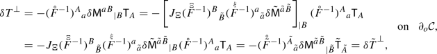
where
 , and the fact that \(\Xi \) (and \(\xi \)) fixes the boundary of the cloak \(\partial _o{\mathcal {C}}\) to the third order were used.
Note that in the case of a general isotropic energy function for the virtual plate \({\pmb {{\mathbb {B}}}}\), \(\mathring{\varvec{{\mathfrak {L}}}}\), and \(\mathring{\varvec{{\mathfrak {B}}}}^\perp \) do not vanish and their expressions are given in Remark. 4.16.
Note that \({\mathsf {F}}_{12}\ne 0\), because otherwise, \(\tilde{{\mathsf {b}}}_1=-2\tilde{{\mathsf {b}}}_2\) (from (4.121)), contradicting the positive definiteness of \(\tilde{\pmb {{\mathbb {B}}}}\).
Note that \(\varvec{\eta }\) and \(\varvec{\Lambda }\), respectively, correspond to \({\mathbf {C}}\) and \({\varvec{\Theta }}\) defined previously.

 , and therefore, using a linear cloaking map is not acceptable (see Brun et al.
  , and thus,
 , implies that
 , and the fact that
 References
Al-Attar, D., Crawford, O.: Particle relabelling transformations in elastodynamics. Geophys. J. Int. 205(1), 575–593 (2016)
Angoshtari, A., Yavari, A.: Differential complexes in continuum mechanics. Arch. Ration. Mech. Anal. 216(1), 193–220 (2015)
Bonnet, O.: Mémoire sur la théorie des surfaces applicables sur une surface donnée. deuxième partie. Gauthier-Villars, Paris (1867)
Brun, M., Guenneau, S., Movchan, A.B.: Achieving control of in-plane elastic waves. Appl. Phys. Lett. 94(6), 061903 (2009)
Brun, M., Colquitt, D., Jones, I., Movchan, A., Movchan, N.: Transformation cloaking and radial approximations for flexural waves in elastic plates. New J. Phys. 16(9), 093020 (2014)
Bryan, K., Leise, T.: Impedance imaging, inverse problems, and Harry Potter’s cloak. SIAM Rev. 52(2), 359–377 (2010)
Capovilla, R., Guven, J.: Stresses in lipid membranes. J. Phys. A Math. Gen. 35(30), 6233 (2002)
Chen, H., Chan, C.T.: Acoustic cloaking in three dimensions using acoustic metamaterials. Appl. Phys. Lett. 91(18), 183518 (2007)
Climente, A., Torrent, D., Sánchez-Dehesa, J.: Analysis of flexural wave cloaks. AIP Adv. 6(12), 121704 (2016)
Colquitt, D.J., Jones, I.S., Movchan, N.V., Movchan, A.B., Brun, M., McPhedran, R.C.: Making waves round a structured cloak: lattices, negative refraction and fringes. Proc. R. Soc. A 469, 2157 (2013)
Colquitt, D.J., Brun, M., Gei, M., Movchan, A.B., Movchan, N.V., Jones, I.S.: Transformation elastodynamics and cloaking for flexural waves. J. Mech. Phys. Solids 72, 131–143 (2014)
Cummer, S.A., Popa, B.-I., Schurig, D., Smith, D.R., Pendry, J., Rahm, M., Starr, A.: Scattering theory derivation of a 3D acoustic cloaking shell. Phys. Rev. Lett. 100(2), 024301 (2008a)
Cummer, S.A., Rahm, M., Schurig, D.: Material parameters and vector scaling in transformation acoustics. New J. Phys. 10(11), 115025 (2008b)
Darabi, A., Zareei, A., Alam, M.-R., Leamy, M.J.: Experimental demonstration of an ultrabroadband nonlinear cloak for flexural waves. Phys. Rev. Lett. 121(17), 174301 (2018)
Deserno, M.: Notes on Differential Geometry with Special Emphasis on Surfaces in \({\mathbb{R}}^3\), pp. 1–64. UCLA, Los Angeles (2004)
do Carmo, M.P.: Riemannian Geometry. Mathematics: Theory & Applications. Birkhäuser, Boston (1992)
Ergin, T., Stenger, N., Brenner, P., Pendry, J.B., Wegener, M.: Three-dimensional invisibility cloak at optical wavelengths. Science 328(5976), 337–339 (2010)
Ericksen, J.L., Truesdell, C.: Exact theory of stress and strain in rods and shells. Arch. Ration. Mech. Anal. 1(1), 295–323 (1957)
Fachinotti, V.D., Peralta, I., Albanesi, A.E.: Optimization-based design of an elastostatic cloaking device. Sci. Rep. 8(1), 1–8 (2018)
Farhat, M., Enoch, S., Guenneau, S., Movchan, A.B.: Broadband cylindrical acoustic cloak for linear surface waves in a fluid. Phys. Rev. Lett. 101(13), 134501 (2008)
Farhat, M., Guenneau, S., Enoch, S.: Ultrabroadband elastic cloaking in thin plates. Phys. Rev. Lett. 103(2), 024301 (2009a)
Farhat, M., Guenneau, S., Enoch, S., Movchan, A.B.: Cloaking bending waves propagating in thin elastic plates. Phys. Rev. B 79(3), 033102 (2009b)
Fox, D., Raoult, A., Simo, J.C.: A justification of nonlinear properly invariant plate theories. Arch. Ration. Mech. Anal. 124(2), 157–199 (1993)
Friesecke, G., James, R.D., Müller, S.: A theorem on geometric rigidity and the derivation of nonlinear plate theory from three-dimensional elasticity. Commun. Pure Appl. Math. A 55(11), 1461–1506 (2002)
Greenleaf, A., Lassas, M., Uhlmann, G.: On nonuniqueness for Calderón’s inverse problem. Math. Res. Lett. 10 (2003a)
Greenleaf, A., Lassas, M., Uhlmann, G.: Anisotropic conductivities that cannot be detected by EIT. Physiol. Meas. 24(2), 413 (2003b)
Greenleaf, A., Kurylev, Y., Lassas, M., Uhlmann, G.: Full-wave invisibility of active devices at all frequencies. Commun. Math. Phys. 275(3), 749–789 (2007)
Greenleaf, A., Kurylev, Y., Lassas, M., Uhlmann, G.: Cloaking devices, electromagnetic wormholes, and transformation optics. SIAM Rev. 51(1), 3–33 (2009a)
Greenleaf, A., Kurylev, Y., Lassas, M., Uhlmann, G.: Invisibility and inverse problems. Bull. Am. Math. Soc. 46(1), 55–97 (2009b)
Guenneau, S., Puvirajesinghe, T.M.: Fick’s second law transformed: one path to cloaking in mass diffusion. J. R. Soc. Interface 10(83), 20130106 (2013)
Guenneau, S., Amra, C., Veynante, D.: Transformation thermodynamics: cloaking and concentrating heat flux. Opt. Express 20(7), 8207–8218 (2012)
Gurney, C.: An Analysis of the Stresses in a Flat Plate with a Reinforced Circular Hole Under Edge Forces. Reports and Memoranda. H.M. Stationery Office (1938)
Han, T., Bai, X., Thong, J.T., Li, B., Qiu, C.-W.: Full control and manipulation of heat signatures: cloaking, camouflage and thermal metamaterials. Adv. Mater. 26(11), 1731–1734 (2014)
Hicks, N.J.: Notes on Differential Geometry. van Nostrand, Amsterdam (1965)
Hostos, J.C.Á., Fachinotti, V.D., Peralta, I.: Metamaterial for elastostatic cloaking under thermal gradients. Sci. Rep. 9(1), 3614 (2019)
Jones, I., Brun, M., Movchan, N., Movchan, A.: Singular perturbations and cloaking illusions for elastic waves in membranes and Kirchhoff plates. Int. J. Solids Struct. 69, 498–506 (2015)
Kadianakis, N., Travlopanos, F.: Kinematics of hypersurfaces in Riemannian manifolds. J. Elast. 111(2), 223–243 (2013)
Kadianakis, N., Travlopanos, F.I.: Infinitesimally affine deformations of a hypersurface. Math. Mech. Solids 23(2), 209–220 (2018)
Kadic, M., Bückmann, T., Schittny, R., Wegener, M.: Metamaterials beyond electromagnetism. Rep. Prog. Phys. 76(12), 126501 (2013)
Kadic, M., Bückmann, T., Schittny, R., Wegener, M.: Experiments on cloaking in optics, thermodynamics and mechanics. Philos. Trans. A 373(2049), 20140357 (2015)
Koschny, T., Soukoulis, C.M., Wegener, M.: Metamaterials in microwaves, optics, mechanics, thermodynamics, and transport. J. Opt. 19(8), 084005 (2017)
Le Dret, H., Raoult, A.: Le modèle de membrane non linéaire comme limite variationnelle de l’élasticité non linéaire tridimensionnelle. Comptes rendus de l’Académie des sciences. Série 1, Mathématique 317(2), 221–226 (1993)
Lee, J.M.: Riemannian Manifold. An Introduction to Curves. Springer, New York (1997)
Lekhnitskii, S.: Anisotropic Plates. Gordon and Breach, London (1968)
Lenz, P., Lipowsky, R.: Stability of droplets and channels on homogeneous and structured surfaces. Eur. Phys. J. E 1(2–3), 249–262 (2000)
Leonhardt, U.: Optical conformal mapping. Science 312(5781), 1777–1780 (2006)
Leonhardt, U., Philbin, T.: Geometry and Light: The Science of Invisibility. Courier Corporation, New York (2012)
Liu, M., Zhu, W.: Nonlinear transformation-based broadband cloaking for flexural waves in elastic thin plates. J. Sound Vib. 445, 270–287 (2019)
Lods, V., Miara, B.: Nonlinearly elastic shell models: a formal asymptotic approach II. The flexural model. Arch. Ration. Mech. Anal. 142(4), 355–374 (1998)
Mansfield, E.H.: Neutral holes in plane sheet—reinforced holes which are elastically equivalent to the uncut sheet. Q. J. Mech. Appl. Math. 6(3), 370 (1953)
Marsden, J.E., Hughes, T.J.R.: Mathematical Foundations of Elasticity. Dover, New York (1983)
Marsden, J.E., Ratiu, T.S.: Introduction to Mechanics and Symmetry, vol. 17. Springer, Berlin (2013)
Mazzucato, A.L., Rachele, L.V.: Partial uniqueness and obstruction to uniqueness in inverse problems for anisotropic elastic media. J. Elast. 83(3), 205–245 (2006)
Milton, G.W., Briane, M., Willis, J.R.: On cloaking for elasticity and physical equations with a transformation invariant form. New J. Phys. 8(10), 248 (2006)
Misseroni, D., Colquitt, D.J., Movchan, A.B., Movchan, N.V., Jones, I.S.: Cymatics for the cloaking of flexural vibrations in a structured plate. Sci. Rep. 6, 23929 (2016)
Naghdi, P.M.: The Theory of Shells and Plates, pp. 425–640. Springer, Berlin (1973)
Nishikawa, S.: Variational Problems in Geometry. American Mathematical Society, Providence (2002)
Norris, A.N.: Acoustic cloaking theory. Proc. R. Soc. Lond. A 464(2097), 2411–2434 (2008)
Parnell, W.J.: Nonlinear pre-stress for cloaking from antiplane elastic waves. Proc. R. Soc. A 468(2138), 563–580 (2012)
Pendry, J.B., Schurig, D., Smith, D.R.: Controlling electromagnetic fields. Science 312(5781), 1780–1782 (2006)
Pomot, L., Bourgeois, S., Payan, C., Remillieux, M., Guenneau, S.: On form invariance of the Kirchhoff-Love plate equation (2019). arXiv preprint arXiv:1901.00067
Reissner, H., Morduchow, M.: Reinforced circular cutouts in plane sheets. Technical Report Technical Note No. 1852 (1949)
Sadik, S., Angoshtari, A., Goriely, A., Yavari, A.: A geometric theory of nonlinear morphoelastic shells. J. Nonlinear Sci. 26, 929–978 (2016)
Schurig, D., Mock, J., Justice, B., Cummer, S.A., Pendry, J.B., Starr, A., Smith, D.: Metamaterial electromagnetic cloak at microwave frequencies. Science 314(5801), 977–980 (2006)
Simo, J., Marsden, J.: Stress tensors, Riemannian metrics and the alternative descriptions in elasticity. In: Ciarlet, P.G., Roseau, M (eds.) Trends and Applications of Pure Mathematics to Mechanics, pp. 369–383. Springer, Berlin (1984)
Simo, J.C., Marsden, J.E., Krishnaprasad, P.S.: The Hamiltonian structure of nonlinear elasticity: the material and convective representations of solids, rods, and plates. Arch. Ration. Mech. Anal. 104(2), 125–183 (1988)
Sklan, S.R., Pak, R.Y., Li, B.: Seismic invisibility: elastic wave cloaking via symmetrized transformation media. New J. Phys. 20(6), 063013 (2018)
Steigmann, D.J.: On the frame invariance of linear elasticity theory. Z. Angew. Math. Phys. 58(1), 121–136 (2007)
Stenger, N., Wilhelm, M., Wegener, M.: Experiments on elastic cloaking in thin plates. Phys. Rev. Lett. 108(1), 014301 (2012)
Syvret, F., Al-Attar, D.: Thermoelastic cloaking and the breaking of invisibility (2019). arXiv preprint arXiv:1903.06664
Timoshenko, S.P., Woinowsky-Krieger, S.: Theory of Plates and Shells. McGraw-Hill, New York (1959)
Valagiannopoulos, C.: Perfect quantum cloaking of tilted cylindrical nanocavities. Phys. Rev. B 101(19), 195301 (2020)
Valagiannopoulos, C.A., Askarpour, A.N., Alu, A.: Aharonov–Bohm detection of two-dimensional magnetostatic cloaks. Phys. Rev. B 92(22), 224414 (2015)
Verpoort, S.: The geometry of the second fundamental form: Curvature properties and variational aspects. PhD thesis, Katholieke Universiteit Leuven (2008)
Yavari, A., Golgoon, A.: Nonlinear and linear elastodynamic transformation cloaking. Arch. Ration. Mech. Anal. 234(1), 211–316 (2019)
Yavari, A., Ozakin, A.: Covariance in linearized elasticity. Z. Angew. Math. Phys. 59(6), 1081–1110 (2008)
Yavari, A., Marsden, J.E., Ortiz, M.: On spatial and material covariant balance laws in elasticity. J. Math. Phys. 47(4), 042903 (2006)
Yavari, A., Ozakin, A., Sadik, S.: Nonlinear elasticity in a deforming ambient space. J. Nonlinear Sci. 26(6), 1651–1692 (2016)
Zareei, A., Alam, M.-R.: Broadband cloaking of flexural waves. Phys. Rev. E 95, 063002 (2017)
Zhang, S., Genov, D.A., Sun, C., Zhang, X.: Cloaking of matter waves. Phys. Rev. Lett. 100(12), 123002 (2008)
Zhou, X., Hu, G., Lu, T.: Elastic wave transparency of a solid sphere coated with metamaterials. Phys. Rev. B 77(2), 024101 (2008)
Acknowledgements
This research was supported by ARO W911NF-18-1-0003 (Drs. Daniel P. Cole and David Stepp). A.G. benefited from discussions with Fabio Sozio, Arzhang Angoshtari, Amirhossein Tajdini, and Souhayl Sadik.
Author information
Authors and Affiliations
Corresponding author
Additional information
Communicated by Robert V. Kohn.
Dedicated to Professor J.N. Reddy on the occasion of his 75th birthday.
Publisher's Note
Springer Nature remains neutral with regard to jurisdictional claims in published maps and institutional affiliations.
Appendices
Appendix A: Variations of the Right Cauchy–Green Deformation Tensor, the Unit Normal Vector Field, and the Second Fundamental Form
In this appendix, we discuss the derivation of the variations of the right Cauchy–Green deformation tensor \({\mathbf {C}}\), the unit normal vector field (of the deformed shell) \(\varvec{{\mathcal {N}}}\), and \({\varvec{\Theta }}\) used in obtaining the Euler–Lagrange equations in Sect. 3 (see also Capovilla and Guven 2002; Kadianakis and Travlopanos 2013, 2018).
Lie derivative. Let \({\mathbf {w}}:{\mathcal {U}}\rightarrow T{\mathcal {S}}\) be a \(C^1\) vector field, where \({\mathcal {U}} \subset {\mathcal {S}}\) is an open neighborhood. A curve \(\alpha :I \rightarrow {\mathcal {S}}\), where I is an open interval, is an integral curve of \({\mathbf {w}}\) provided that \(\frac{d \alpha (t)}{dt}={\mathbf {w}}(\alpha (t)),~\forall ~t \in I\). Consider a time-dependent vector field \({\mathbf {w}}:{\mathcal {S}}\times I\rightarrow T{\mathcal {S}}\), where I is some open interval. The collection of maps \(\psi _{\tau ,t}\) is the flow of \({\mathbf {w}}\) if for each t and x, \(\tau \mapsto \psi _{\tau ,t}(x)\) is an integral curve of \({\mathbf {w}}_t\), i.e., \(\frac{d}{d\tau }\psi _{\tau ,t}(x)={\mathbf {w}}(\psi _{\tau ,t}(x),\tau )\), and \(\psi _{t,t}(x)=x\). Assume that \({\mathbf {t}}\) is a time-dependent tensor field on \({\mathcal {S}}\), i.e., \({\mathbf {t}}_t(x)={\mathbf {t}}(x,t)\) is a tensor. The Lie derivative of \({\mathbf {t}}\) with respect to \({\mathbf {w}}\) is defined as
Note that \(\psi _{\tau ,t}\) maps \({\mathbf {t}}_t\) to \({\mathbf {t}}_{\tau }\). Therefore, to calculate the Lie derivative one drags \({\mathbf {t}}\) along the flow of \({\mathbf {w}}\) from \(\tau \) to t and then differentiates the Lie dragged tensor with respect to \(\tau \). The autonomous Lie derivative of \({\mathbf {t}}\) with respect to \({\mathbf {w}}\) is defined as
Hence, \({\mathbf {L}}_{{\mathbf {w}}}{\mathbf {t}}=\partial {\mathbf {t}}/\partial t+{\mathfrak {L}}_{{\mathbf {w}}}{\mathbf {t}}\). The Lie derivative for a scalar f is given by \({\mathbf {L}}_{{\mathbf {w}}}f=\partial f/\partial t+{\mathbf {w}}[f]\). In a coordinate chart \(\{x^a\}\), this is written as, \({\mathbf {L}}_{{\mathbf {w}}}f=\frac{\partial f}{\partial t}+\frac{\partial f}{\partial x^a}w^a\). For a vector \({\mathbf {u}}\), it can be shown that \({\mathbf {L}}_{{\mathbf {w}}}{\mathbf {u}}=\frac{\partial {\mathbf {w}}}{\partial t}+[{\mathbf {w}},{\mathbf {u}}]\). If \(\nabla \) is a torsion-free connection, then \([{\mathbf {w}},{\mathbf {u}}]=\nabla _{{\mathbf {w}}}{\mathbf {u}}-\nabla _{{\mathbf {u}}}{\mathbf {w}}\), and thus, \({\mathbf {L}}_{{\mathbf {w}}}{\mathbf {u}}=\frac{\partial {\mathbf {w}}}{\partial t}+\nabla _{{\mathbf {w}}}{\mathbf {u}}-\nabla _{{\mathbf {u}}}{\mathbf {w}}\).
The rate of deformation tensor for shells is defined as (Marsden and Hughes 1983)
where the spatial velocity is decomposed into the normal and tangential components as \({\mathbf {v}}={\mathbf {v}}^\top +v^\perp {\mathbf {n}}\). In components
Note that
Therefore,
Knowing that \(\varphi _t^*({\mathbf {L}}_{{\mathbf {v}}}{\mathbf {g}})=2{\mathbf {D}}^\flat \) (see, e.g., Marsden and Hughes 1983; Simo and Marsden 1984), one obtains
Thus, \({\mathbf {L}}_{\delta \varphi }{\mathbf {g}}={\mathbf {L}}_{\delta \varphi ^\top }{\mathbf {g}}-2\,\delta \varphi ^\perp \,\varvec{\theta }\), and hence, \(\delta {\mathbf {C}}^\flat =\varphi ^*_t({\mathbf {L}}_{\delta \varphi }{\mathbf {g}})=\varphi ^*_t\,{\mathbf {L}}_{\delta \varphi ^\top }{\mathbf {g}}-2\,\delta \varphi ^\perp \,{\varvec{\Theta }}\). Also note that
Hence, in components, one obtains
Or
Therefore, (3.11) is implied.
The covariant derivative of \({\mathbf {v}}\) is computed as
Using the relations (2.3) and (2.5) in the ambient space, one obtains
In components
Similarly, one can write
Note that for an arbitrary vector field \({\mathbf {W}}={{\mathbf {W}}}^\top +W^\perp \varvec{{\mathcal {N}}}\) defined on a surface embedded in \({\mathbb {R}}^3\), the tangential and normal components of the covariant derivative with respect to the surface coordinates are similarly given by
Therefore, \({\bar{\nabla }}^{\bar{{\mathbf {g}}}}{\mathbf {W}}=({\bar{\nabla }}^{\bar{{\mathbf {g}}}}{\mathbf {W}})^\top +({\bar{\nabla }}^{\bar{{\mathbf {g}}}}{\mathbf {W}})^\perp \), in components reads
Thus, one can use (A.16)\(_1\) to write the variation of the deformation gradient in components as
Therefore, (3.60) follows. At any time t, the deformation map \(\varphi _t:{\mathcal {H}}\rightarrow {\mathcal {S}}\) is a smooth embedding of the (undeformed) shell into the ambient space. For each \(X\in {\mathcal {H}}\), let \(T\varphi _t(X):T_X{\mathcal {H}}\rightarrow T_{\varphi _t(X)}{\mathcal {S}}\) be the tangent of \(\varphi _t\) at X. The variation of the unit normal vector \(\varvec{{\mathcal {N}}}_{\epsilon }={\mathbf {n}}_{\epsilon }\circ \varphi _{\epsilon ,t}\) is defined as
In order to compute the variation, let \({\mathbf {W}}\) be a vector field in \({\mathcal {S}}\) tangent to \(\varphi _t({\mathcal {H}})\) and note that
From (A.12), one obtains
Therefore,
where the second equality is a consequence of the metric compatibility of \({\bar{\nabla }}^{\bar{{\mathbf {g}}}}\) (2.4). By arbitrariness of \({\mathbf {W}}\), we have
In components
Hence, (3.19) and (3.20) are followed. Note that \(\delta {\varvec{\Theta }}^\flat =\varphi ^*_t({\mathbf {L}}_{\delta \varphi } \varvec{\theta })\), where \( {\mathbf {L}}_{\delta \varphi }\varvec{\theta }={\mathbf {L}}_{\delta \varphi ^\top }\varvec{\theta }-\delta \varphi ^\perp \mathbf {III}+\mathrm {Hess}_{\delta \varphi ^\perp }, \) i.e.,
where for \({\varvec{x}},{\varvec{y}}\in {\mathcal {X}}(\varphi ({\mathcal {H}}))\), the third fundamental form of the deformed hypersurface \(\mathbf {III}\) and the Hessian of \(\delta \varphi ^\perp \), i.e., \(\mathrm {Hess}_{\delta \varphi ^\perp }\) are given by (3.15) and (3.16). The Lie derivative with respect to the tangential component of the variation field is given in components by (see, e.g., Marsden and Hughes 1983, p.97)
Therefore, in components, one can write the variation of \({\varvec{\Theta }}^\flat \) as
Using (A.17) and the fact that \(\Theta _{AB}=F^a{}_AF^b{}_B\theta _{ab}\), one obtains the variation of \(\varvec{\theta }^\flat \) as
Hence, (3.17) and (3.75) are obtained.
Proof of the relation (A.24). Here, we give a proof of the relation (A.24), see also (Capovilla and Guven 2002; Lenz and Lipowsky 2000; Deserno 2004). For the sake of simplicity, we assume that the surface is embedded in three-dimensional Euclidean space. For this proof, we adopt a notation different from the rest of the paper. Let us consider an embedded surface denoted by \(\Sigma \) in \({\mathbb {R}}^3\). The surface geometry is locally described by three functions \({\mathbf {x}}(x^1,x^2,x^3)={\mathbf {X}}(\nu ^\alpha )\) in the Cartesian coordinates \(\{x^1,x^2,x^3\}\) such that \(\{\nu ^\alpha \}\), \(\alpha =1,2\), is a local coordinate chart on the surface. Let us define two tangent vectors \({\mathbf {e}}_{\alpha }={\partial }{\mathbf {X}}/{\partial \nu ^\alpha }\) on the surface. We note that the surface geometry is completely described by its induced metric \(\eta _{\alpha \beta }\) and its induced second fundamental form \(\Lambda _{\alpha \beta }\).Footnote 43 Note that \(\eta _{\alpha \beta }={\mathbf {e}}_{\alpha }\cdot {\mathbf {e}}_{\beta }\), where “\(\cdot \)” denotes the dot product in \({\mathbb {R}}^3\). Let us denote the surface covariant derivative with \(\nabla _\alpha \). Then, one can write the Gauss–Weingarten equations as \(\nabla _{\alpha }{\mathbf {e}}_{\beta }=\Lambda _{\alpha \beta }{\mathbf {n}}\), and \(\nabla _{\alpha }{\mathbf {n}}=-\Lambda _{\alpha \beta }{\mathbf {e}}^{\beta }\), where \({\mathbf {n}}\) is the unit normal vector to the surface. Let us consider the deformation of the embedding functions of the surface \({\mathbf {X}}(\nu )\rightarrow {\mathbf {X}}(\nu )+\delta {\mathbf {X}}(\nu )\) such that the variation field \(\delta {\mathbf {X}}\) is decomposed into the tangential and normal components as \(\delta {\mathbf {X}}=(\psi ^\top )^\alpha {\mathbf {e}}_{\alpha }+\psi ^\perp {\mathbf {n}}\). Using the relation \(\Lambda _{\alpha \beta }={\mathbf {n}}\cdot \nabla _{\alpha }{\mathbf {e}}_{\beta }\), one may write
Knowing that the variation of the unit normal vector is purely tangential, the first term vanishes, i.e., \(\delta {\mathbf {n}}\cdot \nabla _{\alpha }\nabla _{\beta }{\mathbf {X}}=\delta {\mathbf {n}}\cdot \nabla _{\alpha }{\mathbf {e}}_{\beta }=\Lambda _{\alpha \beta }(\delta {\mathbf {n}})\cdot {\mathbf {n}}=0\). After some simplification and using the Codazzi–Mainardi equation \(\nabla _{\alpha }\Lambda _{\beta \gamma }=\nabla _{\beta }\Lambda _{\alpha \gamma }\), one obtains
Notice that the first three terms correspond to the Lie derivative of the induced second fundamental form with respect to the tangential component of the variation field, and thus, (A.29) can be rewritten as
Therefore, (A.24) follows.
Appendix B: The Euler–Lagrange Equations of Elastic Shells
In this appendix, we discuss the derivation of the Euler–Lagrange equations. Substituting (3.8), (3.12), (3.18), and (3.20) into (3.6), one obtains
After some simplification, we have
This can further be simplified to read
We assume that \(\delta \varphi (X,t_0)=\delta \varphi (X,t_1)=0\). Using Stokes’ theorem, we have
where \({{{\mathbf {\mathsf{{T}}}}}}\) is the outward vector field normal to the boundary curve \(\partial {\mathcal {H}}\). Knowing that \(\delta \varphi ^\top \), \(\delta \varphi ^\perp \), and \({\mathbf {d}}(\delta \varphi ^\perp )\) are arbitrary, from (B.4) the Euler–Lagrange equations (3.21) along with the boundary conditions (3.22) are obtained.
Rights and permissions
About this article

Cite this article
Golgoon, A., Yavari, A. Transformation Cloaking in Elastic Plates. J Nonlinear Sci 31, 17 (2021). https://doi.org/10.1007/s00332-020-09660-7
Received:
Accepted:
Published:
DOI: https://doi.org/10.1007/s00332-020-09660-7