Squared error-based shrinkage estimators of discrete probabilities and their application to variable selection

Abstract

In the paper we consider a new approach to regularize the maximum likelihood estimator of a discrete probability distribution and its application in variable selection. The method relies on choosing a parameter of its convex combination with a low-dimensional target distribution by minimising the squared error (SE) instead of the mean SE (MSE). The choice of an optimal parameter for every sample results in not larger MSE than MSE for James–Stein shrinkage estimator of discrete probability distribution. The introduced parameter is estimated by cross-validation and is shown to perform promisingly for synthetic dependence models. The method is applied to introduce regularized versions of information based variable selection criteria which are investigated in numerical experiments and turn out to work better than commonly used plug-in estimators under several scenarios.

Appendices

A Proof of Eq. (4)

Proof

First recall the form of $\lambda _{MSE}$ in (4):

$$\begin{aligned} \lambda _{MSE}= & {} \frac{\sum _x \Big (\mathrm{Var}({{\hat{p}}}^{(2)}(x))- \mathrm{Cov}( {{\hat{p}}}^{(1)}(x), {{\hat{p}}}^{(2)}(x))\Big )}{\sum _x {{\,\mathrm{{\mathbb {E}}}\,}}({{\hat{p}}}^{(1)}(x)- {{\hat{p}}}^{(2)}(x))^2}. \end{aligned}$$

Similarly to the proof of Lemma 1, we notice that $MSE(\lambda )$ is a quadratic function of $\lambda$:

$$\begin{aligned} MSE(\lambda )= & {} {{\,\mathrm{{\mathbb {E}}}\,}}\bigg (\sum _x (p(x)-{{\hat{p}}}_\lambda (x))^2 \bigg )= {{\,\mathrm{{\mathbb {E}}}\,}}\bigg (\sum _x \Big [\lambda ^2\left( {{\hat{p}}}^{(1)}(x) - {{\hat{p}}}^{(2)}(x)\right) ^2 \nonumber \\&\quad - 2\lambda \left( p(x)-{{\hat{p}}}^{(2)}(x)\right) \left( {{\hat{p}}}^{(1)}(x)- {{\hat{p}}}^{(2)}(x)\right) + \left( p(x) - {{\hat{p}}}^{(2)}(x)\right) ^2\Big ]\bigg ).\nonumber \\ \end{aligned}$$

(37)

Therefore, we obtain

$$\begin{aligned} \lambda _{MSE}=\frac{\sum _x {{\,\mathrm{{\mathbb {E}}}\,}}\left( p(x)-{{\hat{p}}}^{(2)}(x)\right) \left( {{\hat{p}}}^{(1)}(x)- {{\hat{p}}}^{(2)}(x)\right) }{\sum _x {{\,\mathrm{{\mathbb {E}}}\,}}\left( {{\hat{p}}}^{(1)}(x)- {{\hat{p}}}^{(2)}(x)\right) ^2} \end{aligned}$$

(38)

and as ${{\,\mathrm{{\mathbb {E}}}\,}}{{\hat{p}}}^{(2)}(x) = p(x)$, we have

$$\begin{aligned}\mathrm{Var}({{\hat{p}}}^{(2)}(x))={{\,\mathrm{{\mathbb {E}}}\,}}\left( {{\hat{p}}}^{(2)}(x) - p(x)\right) {{\hat{p}}}^{(2)}(x)\end{aligned}$$

and

$$\begin{aligned}\mathrm{Cov}({{\hat{p}}}^{(1)}(x),{{\hat{p}}}^{(2)}(x))={{\,\mathrm{{\mathbb {E}}}\,}}\left( {{\hat{p}}}^{(2)}(x) - p(x)\right) {{\hat{p}}}^{(1)}(x).\end{aligned}$$

$\square$

B Proof of Theorem 1

Proof

As ${{\hat{p}}}^{(2)}(x,y)$ is the maximum likelihood estimator of p(x, y), its variance and second moment is well known and we omit the proof. We prove first corrected formula for ${{\,\mathrm{{\mathbb {E}}}\,}}\left( p^{(1)}(x, y) \right) ^2$. We have

$$\begin{aligned} {{\,\mathrm{{\mathbb {E}}}\,}}\left( {{\hat{p}}}^{(1)}(x, y) \right) ^2 = \frac{1}{n^4}{{\,\mathrm{{\mathbb {E}}}\,}}\left[ \sum \limits _{i} {\mathbb {I}}(X_i = x)\sum \limits _{i'} {\mathbb {I}}(X_{i'} = x)\sum \limits _{j} {\mathbb {I}}(Y_j = y)\sum \limits _{j'} {\mathbb {I}}(Y_{j'} = y) \right] . \end{aligned}$$

The contribution to the expected value of the summands on RHS depends on the number of elements of the set $A_1=\{i, i', j, j'\}$.

• $|A_1| = 1$ ($i=j=i'=j'$)

  The contribution is $np(x, y)/n^4$.

• $|A_1| = 2$

  We have four cases:

  • 1. $i = i', j = j', i \ne j$

    $n(n-1)p(x)p(y)/n^4$

  • 2. $i = j, i' = j', i \ne i'$ or $i = j', i = j', i \ne i'$. These two cases have the same contribution which equals:

    $n(n-1)p^2(x, y)/n^4$

  • 3. $i = i' = j, j \ne j'$ or $i = i' = j', j \ne j'$

    $n(n-1)p(x, y)p(y)/n^4$

  • 4. $i = j' = j, i \ne i'$ or $i' = j = j', i \ne i'$

    $n(n-1)p(x, y)p(x)/n^4$

• $|A| = 3$

  We have three cases:

  • 1. $i \ne i', j = j', j \ne i, j \ne i'$

    $n(n-1)(n-2)p^2(x)p(y)/n^4$

  • 2. $i = i', j \ne j', i \ne j, i \ne j'$

    $n(n-1)(n-2)p(x)p^2(y)/n^4$

  • 3. $i = j, i \ne i', j \ne j', i \ne j'$ (there are four cases like this—the remaining three have pairwise unequal indices except for one pair from $\{(i, j')$, $(i', j)$, $(i', j')\}$)

    $n(n-1)(n-2)p(x, y)p(x)p(y)/n^4$

• $|A_1| = 4$

  $n(n-1)(n-2)(n-3)p^2(x)p^2(y)/n^4$

Summing up all of the terms we obtain the formula in Theorem 2. Similarly, we prove the formula for ${{\,\mathrm{{\mathbb {E}}}\,}}({{\hat{p}}}^{(1)}(x,y){{\hat{p}}}^{(2)}(x,y))$:

$$\begin{aligned} {{\,\mathrm{{\mathbb {E}}}\,}}({{\hat{p}}}^{(1)}(x,y){{\hat{p}}}^{(2)}(x,y)) = \frac{1}{n^3}{{\,\mathrm{{\mathbb {E}}}\,}}\left[ \sum \limits _{i} {\mathbb {I}}(X_i = x)\sum \limits _{j} {\mathbb {I}}(Y_j = y)\sum \limits _{k} {\mathbb {I}}(X_{k} = x){\mathbb {I}}(Y_{k} = y) \right] . \end{aligned}$$

We define $A_2=\{i, j, k\}$, and we have three cases:

• $|A_2| = 1$

  The contribution is $np(x, y)/n^3$.

• $|A_2| = 2$

  We have three cases with corresponding contributions:

  • 1. $i = j, i \ne k$

    $n(n-1)p^2(x,y)/n^3$

  • 2. $i = k, i \ne j$

    $n(n-1)p(x)p(x,y)/n^3$

  • 3. $j = k, j \ne i$

    $n(n-1)p(y)p(x,y)/n^3$

• $|A_2| = 3$

  $n(n-1)(n-2)p(x)p(y)p(x,y)/n^3$

To obtain the formula for covariance of ${{\hat{p}}}^{(1)}(x,y)$ and ${{\hat{p}}}^{(2)}(x,y)$, we need to compute ${{\,\mathrm{{\mathbb {E}}}\,}}{{\hat{p}}}^{(1)}(x,y)$ and then simply use

$$\begin{aligned} \mathrm{Cov}({{\hat{p}}}^{(1)}(x,y),{{\hat{p}}}^{(2)}(x,y)) = {{\,\mathrm{{\mathbb {E}}}\,}}{{\hat{p}}}^{(1)}(x,y){{\hat{p}}}^{(2)}(x,y) - {{\,\mathrm{{\mathbb {E}}}\,}}{{\hat{p}}}^{(1)}(x,y){{\,\mathrm{{\mathbb {E}}}\,}}{{\hat{p}}}^{(2)}(x,y). \end{aligned}$$

To this end we note that

$$\begin{aligned} {{\,\mathrm{{\mathbb {E}}}\,}}{{\hat{p}}}^{(1)}(x,y)&= \frac{1}{n^2}{{\,\mathrm{{\mathbb {E}}}\,}}\left[ \sum \limits _{i} {\mathbb {I}}(X_i = x)\sum \limits _{j} {\mathbb {I}}(Y_j = y)\right] \\&= \left( np(x, y) + n(n-1)p(x)p(y)\right) / n^2. \end{aligned}$$

$\square$

C Asymptotic behaviour of $\lambda$

We state the result analogous to Theorems 3 and 4 which study asymptotic behaviour of theoretical minimisers $\lambda _{MSE}^{U}$ , $\lambda _{SE}^{U}$, $\lambda _{MSE}^{Ind}$ and $\lambda _{SE}^{Ind}$. Note that in cases when the distribution is not uniform or is not a product of its marginals n times theoretical minimisers tend to the same limits as their empirical counterparts. The behaviour of $\lambda _{MSE}^U$ and $\lambda _{SE}^U$ in the uniform case is much simpler as they are equal to 1, whereas $\lambda _{MSE}^{Ind} \rightarrow 1$ in the independent case. The only unresolved case is the behaviour of $\lambda _{SE}^{Ind}$ in the latter case. We include a partial result as the second part of (iv).

Theorem 5

We have the following convergences provided $n\rightarrow \infty$:

• (i) n$\lambda _{MSE}^U \rightarrow c$ when $p(x)\not \equiv 1/m,$ c defined in (22) and $\lambda _{MSE}^U =1$ otherwise;

• (ii) n$\lambda _{SE}^U \rightarrow c$ a.e. when $p(x)\not \equiv 1/m,$ c defined in (22), and $\lambda _{SE}^U =1$ otherwise;

• (iii) n$\lambda _{MSE}^{Ind} \rightarrow c,$ when $p(x,y)\not \equiv p(x)p(y),$ c defined in (27) and $\lambda _{MSE}^{Ind} \rightarrow 1$ otherwise;

• (iv) n $\lambda _{SE}^{Ind} \rightarrow c$ a.e. when $p(x,y)\not \equiv p(x)p(y),$ c defined in (27). Otherwise we have the following representation

  

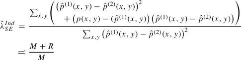
  and ${{\,\mathrm{{\mathbb {E}}}\,}}R =0,$ ${{\,\mathrm{{\mathbb {E}}}\,}}M = O(1/n)$

Proof

We prove the second part of (iv) only as the proofs of the remaining parts are analogous but simpler than those of Theorems 3 and 4. The second part of (ii) follows from checking that the leading terms in the numerator and the denominator of $\lambda _{MSE}^{Ind}$ (of order $n^{-1}$) are the same. We omit the details. In order to prove the second part of (iv) note that representation of $\lambda _{SE}^{Ind}$ follows from a simple calculation. Moreover, using independence we have

$$\begin{aligned} \mathrm{Var}({{\hat{p}}}^{(1)}(x,y))=\bigg (\frac{n-1}{n}p^2(x) +\frac{1}{n}p(x)\bigg )\bigg (\frac{n-1}{n}p^2(y) +\frac{1}{n}p(y)\bigg ) -p^2(x)p^2(y) \end{aligned}$$

and it is seen that it coincides with $\mathrm{Cov}(p^{(1)}(x,y),{{\hat{p}}}^{(2)}(x,y))$ (see Theorem 1). Additionally, it is easily seen that

$$\begin{aligned} \mathrm{Var}({{\hat{p}}}^{(2)}(x,y))- \mathrm{Var}({{\hat{p}}}^{(1)}(x,y))\ge \frac{c_1}{n} \end{aligned}$$

(39)

for some $c_1>0$. Thus we have

$$\begin{aligned} {{\,\mathrm{{\mathbb {E}}}\,}}R= -\sum _{x,y}\mathrm{Var}({{\hat{p}}}^{(1)}(x,y)) + \mathrm{Cov}({{\hat{p}}}^{(1)}(x,y),{{\hat{p}}}^{(2)}(x,y))=0 \end{aligned}$$

whereas

$$\begin{aligned} {{\,\mathrm{{\mathbb {E}}}\,}}M= & {} \sum _{x,y}{{\,\mathrm{{\mathbb {E}}}\,}}\left( {{\hat{p}}}^{(1)}(x,y) - {{\hat{p}}}^{(2)}(x,y)\right) ^2= \sum _{x,y} \Big (\mathrm{Var}({{\hat{p}}}^{(1)}(x,y)) \\&\quad +\mathrm{Var}({{\hat{p}}}^{(2)}(x,y))- 2\mathrm{Cov}({{\hat{p}}}^{(1)}(x,y), {{\hat{p}}}^{(2)}(x,y))\Big ) \ge \frac{c_1}{n} \end{aligned}$$

which ends the proof of the second part of (iv).

$\square$

Remark 4

It follows from the proof of (iv) that in the case when X and Y are independent then

$$\begin{aligned}\mathrm{Var}({{\hat{p}}}^{(2)}(x,y))- \mathrm{Var}({{\hat{p}}}_{\lambda ^{Ind}_{SE}}(x,y))\ge \frac{c_1}{n}\end{aligned}$$

and thus shrinkage estimator has a smaller variance then ML estimator ${{\hat{p}}}^{(2)}$. This is intuitive as ${{\hat{p}}}^{(1)}$ is ML estimator in a smaller model assuming independence of X and Y and it has smaller variance then ${{\hat{p}}}^{(2)}$ [cf. (39)]. This property, which is likely to be preserved for approximate independence, is consistent with an aim of construction of James–Stein shrinkage estimators.

References

Agresti A (2013) Categorical data analysis, 3rd edn. Wiley, Hoboken
Bartoszyński R, Niewiadomska-Bugaj M (1996) Probability and statistical inference, 1st edn. Wiley, New York
Battiti R (1994) Using mutual information for selecting features in supervised neural-net learning. IEEE Trans Neural Netw 5(4):537–550
Borboudakis G, Tsamardinos I (2019) Forward–backward selection with early dropping. J Mach Learn Res 20:1–39
Brown G, Pocock A, Zhao MJ, Luján M (2012) Conditional likelihood maximisation: a unifying framework for information theoretic feature selection. J Mach Learn Res 13(1):27–66
Cover TM, Thomas JA (2006) Elements of information theory. Wiley series in telecommunications and signal processing. Wiley-Interscience, New York
Fleuret F (2004) Fast binary feature selection with conditional mutual information. J Mach Learn Res 5:1531–1555
Guyon I (2003) Design of experiments for the NIPS 2003 variable selection benchmark. Presentation. www.nipsfsc.ecs.soton.ac.uk/papers/NIPS2003-Datasets.pdf
Hall P (1982) Limit theorems for stochastic measures of the accuracy of density estimators. Stoch Process Their Appl 13:11–25
Hall P (1983) Large sample optimality of least-squares crossvalidation in density estimation. Ann Stat 1:1156–1174
Hall P (1984) Central limit theorem for integrated square error of multivariate nonparametric density estimators. J Multivar Anal 14:1–16
Hall P, Marron J (1987) Extent to which least-squares cross-validation minimises integrated square error in nonparametric density estimation. Probab Theory Relat Fields 74:567–581. https://doi.org/10.1007/BF00363516
Hausser J, Strimmer K (2007) Entropy inference and the James–Stein estimator, with applications to nonlinear gene association networks. J Mach Learn Res 10:1469–1484
Hausser J, Strimmer K (2014) Entropy: estimation of entropy, mutual information and related quantities. R package version 1.2.1. CRAN.R-project.org/package=entropy
James W, Stein C (1961) Estimation with quadratic loss. In: Proceedings of fourth Berkeley symposium on mathematical statistics and probability, pp 361–379
Kubkowski M, Mielniczuk J, Teisseyre P (2021) How to gain on power: novel conditional independence tests based on short expansion of conditional mutual information. J Mach Learn Res 22:1–57
Łazȩcka M, Mielniczuk J (2020) Note on Machine Learning (2020) paper by Sechidis et al. Unpublished note
Ledoit O, Wolf M (2003) Improved estimation of the covariance matrix of stock returns with an application to portfolio selection. J Empir Finance 10:603–621
Lewis D (1992) Feature selection and feature extraction for text categorisation. In: Proceedings of the workshop on speech and natural language
Lin D, Tang X (2006) Conditional infomax learning: an integrated framework for feature extraction and fusion. In: Proceedings of the 9th European conference on computer vision—Part I, ECCV’06, pp 68–82
Marron J, Härdle WK (1986) Random approximations to some measures of accuracy in nonparametric curve estimation. J Multivar Anal 20:91–113
Meyer P, Schretter C, Bontempi G (2008) Information-theoretic feature selection in microarray data using variable complementarity. IEEE Sel Top Signal Process 2(3):261–274
Mielniczuk J, Teisseyre P (2019) Stopping rules for mutual information-based feature selection. Neurocomputing 358:255–271
Nelsen R (2006) An introduction to copulas. Springer, New York
Pawluk M, Teisseyre P, Mielniczuk J (2019) Information-theoretic feature selection using high-order interactions. In: Machine learning, optimization, and data science. Springer, pp 51–63
Peng H, Long F, Ding C (2005) Feature selection based on mutual information criteria of max-dependency, max-relevance and min-redundancy. IEEE Trans Pattern Anal Mach Intell 27(1):1226–1238
Rice J (1984) Bandwidth choice for regression estimation. Ann Stat 12(4):1215–1230
Schäffer I, Strimmer K (2005) A shrinkage approach to large-scale covariance matrix estimation and implications for functional genomics. Stat Appl Genet Mol Biol. www.strimmerlab.org/publications/journals/shrinkcov2005.pdf
Scott D (2001) Parametric statistical modeling by minimum integrated square error. Technometrics 43:274–285
Scutari M (2010) Learning Bayesian networks with the bnlearn R package. J Stat Softw 35(3):1–22
Scutari M, Brogini A (2016) Bayesian structure learning with permutation tests. Commun Stat Theory Methods 41(16–17):3233–3243
Sechidis K, Azzimonti L, Pocock A, Corani G, Weatherall J, Brown G (2019) Efficient feature selection using shrinkage estimators. Mach Learn 108:1261–1286
Sechidis K, Azzimonti L, Pocock A, Corani G, Weatherall J, Brown G (2020) Corrigendum to: Efficient feature selection using shrinkage estimators. Mach Learn. https://doi.org/10.1007/s10994-020-05884-6
Stone C (1984) An asymptotically optimal window selection rule for kernel density estimates. Ann Stat 12(4):1285–1297
Sugiyama M, Kanamori T, Suzuki T, Plessis M, Liu S, Takeuchi I (2012) Density-difference estimation. In: Pereira F, Burges CJC, Bottou L, Weinberger KQ (eds) Advances in neural information processing systems. Curran Associates, Inc
Vergara J, Estevez P (2014) A review of feature selection methods based on mutual information. Neural Comput Appl 24(1):175–186
Vinh N, Zhou S, Chan J, Bailey J (2016) Can high-order dependencies improve mutual information based feature selection? Pattern Recognit 53:45–58
Yang HH, Moody J (1999) Data visualization and feature selection: new algorithms for non-Gaussian data. Adv Neural Inf Process Syst 12:687–693
Author information
Authors and Affiliations
Corresponding author
Ethics declarations
Conflict of interest
The authors declare that they have no conflict of interest.
Additional information
Publisher's Note
Springer Nature remains neutral with regard to jurisdictional claims in published maps and institutional affiliations.