Lipschitz embeddings of random sequences

Abstract

We develop a new multi-scale framework flexible enough to solve a number of problems involving embedding random sequences into random sequences. Grimmett et al. (Random Str Algorithm 37(1):85–99, 2010) asked whether there exists an increasing $M$-Lipschitz embedding from one i.i.d. Bernoulli sequence into an independent copy with positive probability. We give a positive answer for large enough $M$. A closely related problem is to show that two independent Poisson processes on $\mathbb R$ are roughly isometric (or quasi-isometric). Our approach also applies in this case answering a conjecture of Szegedy and of Peled (Ann Appl Probab 20:462–494, 2010). Our theorem also gives a new proof to Winkler’s compatible sequences problem. Our approach does not explicitly depend on the particular geometry of the problems and we believe it will be applicable to a range of multi-scale and random embedding problems.

1 Introduction

With his compatible sequences and clairvoyant demon scheduling problems Winkler introduced a fascinating class of dependent or “co-ordinate” percolation type problems (see e.g. [2, 4, 10, 24]). These, and other problems in this class, can be interpreted either as embedding one sequence into another according to certain rules or as oriented percolation problems in $\mathbb Z ^2$ where the sites are open or closed according to random variables on the co-ordinate axes. A natural question of this class posed by Grimmett, Liggett and Richthammer [14] asks whether there exists a Lipshitz embedding of one Bernoulli sequence into another. The following theorem answers the main question of [14].

Theorem 1

Let $\{X_i\}_{i\in \mathbb Z }$ and $\{Y_i\}_{i\in \mathbb Z }$ be independent sequences of independent identically distributed $\hbox {Ber}(\frac{1}{2})$ random variables. For sufficiently large $M$ almost surely there exists a strictly increasing function $\phi :\mathbb Z \rightarrow \mathbb Z$ such that $X_i=Y_{\phi (i)}$ and $1\le \phi (i)-\phi (i-1)\le M$ for all $i$.

The original question of [14] was slightly different asking for a positive probability on the natural numbers with the condition $\phi (0)=0$, which is implied by our theorem (and is equivalent by ergodic theory considerations). Among other results they showed that Theorem 1 fails in the case of $M=2$. In a series of subsequent works Grimmett, Holroyd and their collaborators [6, 10–13, 16] investigated a range of related problems including when one can embed $\mathbb Z ^d$ into site percolation in $\mathbb Z ^D$ and showed that this was possible almost surely for $M=2$ when $D>d$ and the the site percolation parameter was sufficiently large but almost surely impossible for any $M$ when $D \le d$. Recently Holroyd and Martin showed that a comb can be embedded in $\mathbb Z ^2$. Another important series of work in this area involves embedding words into higher dimensional percolation clusters [3, 5, 20, 21]. Despite this impressive progress the question of embedding one random sequence into another remained open. The difficulty lies in the presence of long strings of ones and zeros on all scales in both sequences which must be paired together.

In a similar vein is the question of a rough, (or quasi-), isometry of two independent Poisson processes. Informally, two metric spaces are roughly isometric if their metrics are equivalent up to multiplicative and additive constants. The formal definition, introduced by Gromov [15] in the case of groups and more generally by Kanai [17], is as follows.

Definition 1.1

We say two metric spaces $X$ and $Y$ are roughly isometric with parameters $(M,D,C)$ if there exists a mapping $T:X\rightarrow Y$ such that for any $x_1, x_2 \in X$,

$$\begin{aligned} \frac{1}{M} d_X(x_1,x_2)-D \le d_Y(T(x_1),T(x_2)) \le M d_X(x_1,x_2) + D, \end{aligned}$$

and for all $y\in Y$ there exists $x\in X$ such that $d_Y(T(x),y)\le C$.

Originally Abért [1] asked whether two independent infinite components of bond percolation on a Cayley graph are roughly isometric. Szegedy asked the problem when these sets are independent Poisson process in $\mathbb R$ (see [22] for a fuller description of the history of the problem). The most important progress on this question is by Peled [22] who showed that Poisson processes on $[0,n]$ are roughly isometric with parameter $M=\sqrt{\log n}$. The question of whether two independent Poisson processes on $\mathbb R$ are roughly isometric for fixed $(M,D,C)$ was the main open question of [22]. We prove that this is indeed the case.

Theorem 2

Let $X$ and $Y$ be independent Poisson processes on $\mathbb R$ viewed as metric spaces. There exists $(M,D,C)$ such that almost surely $X$ and $Y$ are $(M,D,C)$-roughly isometric.

Again the challenge is to find a good matching on all scales, in this case to the long gaps in each of the point processes with ones of proportional length in the other. The isometries we find are also weakly increasing answering a further question of Peled [22]. Results of [22] show that Theorem 2 applies to one dimensional site percolation as well.

Our final result is the compatible sequence problem of Winkler. Given two independent sequence $\{X_i\}_{i\in \mathbb N }$ and $\{Y_i\}_{i\in \mathbb N }$ of independent identically distributed $\hbox {Ber}(q)$ random variables we say they are compatible if after removing some zeros from both sequences, there is no index with a 1 in both sequence. Equivalently there exist increasing subsequences $k_1,k_2,\ldots ,$ (respectively $k_1^{\prime }\ldots$) such that if $X_j=1$ then $j=k_i$ for some $i$ (resp. if $Y_j=1$ then $j=k_i^{\prime }$) so that for all $i$, we have $X_{k_i}Y_{k_i^{\prime }}=0$. We give a new proof of the following result of Gács [7].

Theorem 3

For sufficiently small $q>0$ two independent $\hbox {Ber}(q)$ sequences $\{X_i\}_{i\in \mathbb N }$ and $\{Y_i\}_{i\in \mathbb N }$ are compatible with positive probability.

Our proof is different and we believe more transparent enabling us to state a concise induction step (see Theorem 4.1). Other recent progress was made on this problem by Kesten et al. [18] constructing sequences which are compatible with a random sequence with positive probability.

Each of these results follows from an abstract theorem in the next section which applies to a range of different models. The novelty of our multi-scale approach is that, as far as possible, we ignore the anatomy of what makes different configurations difficult to embed and instead consider simply the probability that they can be embedded into a random block proving recursive power-law estimates for these quantities. It is thus well suited to addressing even more challenging embedding problems such as random embeddings or rough isometries of higher dimensional percolation where to give a description of bad configurations becomes increasingly complex. We expect that our framework will find uses in a range of other multi-scale problems.

Independent results Two other researchers have also solved some of these problems independently. Vladas Sidoravicius [23] solved the same set of problems and described his approach to us. His work is based on a different multi-scale approach, proving that for certain choices of parameters $p_1$ and $p_2$ one can see random binary sequence sampled with parameter $p_1$ in the scenery determined by another binary sequence sampled with parameter $p_2$, with positive probability. This generalizes the main theorem of [19] and a slight modification of it then implies Theorems 1, 2 and 3.

Shortly before completing this paper Peter Gács sent us a draft of his paper [9] solving Theorem 1. His approach extends his work on the scheduling problem [8]. The proof is geometric taking a percolation type view and involves a complex multi-scale system of structures. Our work was done completely independently of both.

1.1 General theorem

To apply to a range of problems we need to consider larger alphabets of symbols. Let $\mathcal{C }^\mathbb{X }=\{C_1,C_2,\ldots \}$ and $\mathcal{C }^\mathbb{Y }=\{C^{\prime }_1,C^{\prime }_2,\ldots \}$ be a pair of countable alphabets and let $\mu ^\mathbb{X }$ and $\mu ^\mathbb{Y }$ be probability measures on $\mathcal{C }^\mathbb{X }$ and $\mathcal{C }^\mathbb{Y }$ respectively.

We will suppose also that we have a relation $\mathcal R \subseteq \mathcal{C }^\mathbb{X }\times \mathcal{C }^\mathbb{Y }$. If $(C_i,C^{\prime }_k)\in \mathcal R$, we denote this by $C_i \hookrightarrow C^{\prime }_k$. Let $G_0^\mathbb{X }\subseteq \mathcal{C }^\mathbb{X }$ and $G_0^\mathbb{Y }\subseteq \mathcal{C }^\mathbb{Y }$ be two given subsets such that $C_i\in G_0^\mathbb{X }$ and $C^{\prime }_k\in G_0^\mathbb{Y }$ implies $C_i\hookrightarrow C^{\prime }_k$. Symbols in $G_0^\mathbb{X }$ and $G_0^\mathbb{Y }$ will be referred to as “good”.

1.1.1 Definitions

Now let $\mathbb X =(X_1,X_2,\ldots )$ and $\mathbb Y =(Y_1,Y_2,\ldots )$ be two sequences of symbols coming from the alphabets $\mathcal{C }^\mathbb{X }$ and $\mathcal{C }^\mathbb{Y }$ respectively. We will refer to such sequences as an $\mathbb X$-sequence and a $\mathbb Y$-sequence respectively. For $1\le i_1 < i_2$, we call the subsequence $(X_{i_1},X_{i_1+1},\ldots , X_{i_2})$ the “$[i_1,i_2]$-segment” of $\mathbb X$ and denote it by $\mathbb X ^{[i_1,i_2]}$. We call $\mathbb X ^{[i_1,i_2]}$ a “good” segment if $X_i\in G_0^\mathbb{X }$ for $i_1\le i\le i_2$ and similarly for $\mathbb Y$.

Let $R$ be a fixed constant. Let $R_0=2R$, $R_0^{-}=1$, $R_0^{+}=3R^2$.

Definition 1.2

Let $\mathbb X$ and $\mathbb Y$ be sequences as above. Let $X=(X_{a+1},\ldots X_{a+n})$ and $Y=(Y_{a^{\prime }+1},\ldots Y_{a^{\prime }+n^{\prime }})$ be segments of $\mathbb X$ and $\mathbb Y$ respectively. We say $X$ $R$-embeds or $R$-maps into $Y$, denoted $X \hookrightarrow _R Y$if there exists $a=i_0<i_1<i_2<\cdots <i_k=a+n$ and $a^{\prime }=i^{\prime }_0<i^{\prime }_1<i^{\prime }_2< \cdots <i^{\prime }_k=a^{\prime }+n^{\prime }$ satisfying the following conditions.

• 1. For each $r$, either $i_{r+1}-i_{r}=i^{\prime }_{r+1}-i^{\prime }_{r}=1$ or $i_{r+1}-i_{r}=R_0$ or $i^{\prime }_{r+1}-i^{\prime }_{r}=R_0$.

• 2. If $i_{r+1}-i_{r}=i^{\prime }_{r+1}-i^{\prime }_{r}=1$, then $X_{i_{r}+1}\hookrightarrow Y_{i^{\prime }_{r}+1}$.

• 3. If $i_{r+1}-i_{r}=R_0$, then $R_0^{-}\le i^{\prime }_{r+1}-i^{\prime }_{r}\le R_0^{+}$, and both $\mathbb X ^{[i_r+1,i_{r+1}]}$ and $\mathbb Y ^{[i^{\prime }_{r}+1,i^{\prime }_{r+1}]}$ are good segments.

• 4. If $i^{\prime }_{r+1}-i^{\prime }_{r}=R_0$, then $R_0^{-}\le i_{r+1}-i_{r}\le R_0^{+}$, and both $\mathbb X ^{[i_r+1,i_{r+1}]}$ and $\mathbb Y ^{[i^{\prime }_{r}+1,i^{\prime }_{r+1}]}$ are good segments.

We say that $\mathbb X$ $R$-embeds or $R$-maps into $\mathbb Y$, denoted $\mathbb X \hookrightarrow _R \mathbb Y$ if there exists $0=i_0<i_1<i_2<\ldots$ and $0=i^{\prime }_0<i^{\prime }_1<i^{\prime }_2< \ldots$ satisfying the above conditions.

Throughout we will use a fixed $R$ defined in Theorem 4 and will simply refer to mappings and write that $\mathbb X \hookrightarrow \mathbb Y$ (or $X\hookrightarrow Y$) except where it is ambiguous. The following elementary observation is useful. Suppose we have $n_0<n_1<\ldots < n_k$ and $n^{\prime }_0< n^{\prime }_1<\ldots < n^{\prime }_k$ such that $\mathbb X ^{[n_r+1,n_{r+1}]}\hookrightarrow \mathbb Y ^{[n^{\prime }_r+1,n^{\prime }_{r+1}]}$ for $0\le r<k$, then $\mathbb X ^{[n_0+1,n_k]}\hookrightarrow \mathbb Y ^{[n^{\prime }_0+1,n^{\prime }_k]}$.

A key element in our proof is tail estimates on the probability that we can map a block $X$ into a random block $Y$ and so we make the following definition.

Definition 1.3

For $X \in \mathcal{C }^\mathbb{X }$, we define the embedding probability of $X$ as $S_0^\mathbb{X }(X)=\mathbb P (X\hookrightarrow Y|X)$ where $Y\sim \mu ^\mathbb{Y }$. We define $S_0^\mathbb{Y }(Y)$ similarly and suppress the notation $\mathbb X ,\mathbb Y$ when the context is clear.

1.1.2 General theorem

We can now state our general theorem which will imply the main results of the paper as shown in § 2.

Theorem 4

(General Theorem) There exist positive constants $\beta$, $\delta$, $m$, $R$ such that for all large enough $L_0$ the following holds. Let $X\sim \mu ^\mathbb{X }$ and $Y\sim \mu ^\mathbb{Y }$ where $\mu ^\mathbb{X }$ and $\mu ^\mathbb{Y }$ are probability distributions on alphabets such that for all $k\ge L_0$,

$$\begin{aligned} \mu ^\mathbb{X }(\{C_{k+1},C_{k+2},\ldots \})\le \frac{1}{k}, \quad \mu ^\mathbb{Y }(\{C^{\prime }_{k+1},C^{\prime }_{k+2},\ldots \})\le \frac{1}{k}. \end{aligned}$$

(1)

Suppose the following conditions are satisfied

• 1. For all $0< p \le 1-L_0^{-1}$,

  $$\begin{aligned} \mathbb P (S_0^\mathbb{X }(X)\le p)\le p^{m+1}L_0^{-\beta },\quad \mathbb P (S_0^\mathbb{Y }(Y)\le p)\le p^{m+1}L_0^{-\beta }. \end{aligned}$$

  (2)

• 2. Most symbols are “good”,

  $$\begin{aligned} \mathbb P (X\in G_0^\mathbb{X })\ge 1-L_0^{-\delta }, \quad \mathbb P (Y\in G_0^\mathbb{Y })\ge 1-L_0^{-\delta }. \end{aligned}$$

  (3)

Then for $\mathbb X =(X_1,X_2,\ldots )$ and $\mathbb Y =(Y_1,Y_2,\ldots )$, two sequences of i.i.d. symbols with laws $\mu ^\mathbb{X }$ and $\mu ^\mathbb{Y }$ respectively, we have

$$\begin{aligned} \mathbb P (\mathbb X \hookrightarrow _R \mathbb Y )>0. \end{aligned}$$

1.2 Proof outline

The proof makes use of a number of parameters, $\alpha ,\beta ,\delta , m, k_0, R$ and $L_0$ which must satisfy a number of relations described in the next subsection. Our proof is multi-scale and divides the sequences into blocks on a series of doubly exponentially growing length scales $L_j=L_0^{\alpha ^j}$ for $j\ge 0$ and at each of these levels we define a notion of a “good” block. Single characters in the base sequences $\mathbb X$ and $\mathbb Y$ constitute the level 0 blocks.

Suppose that we have constructed the blocks up to level $j$ denoting the sequence as $(X_1^{(j)},X_2^{(j)}\ldots )$. In § 3, we give a construction of $(j+1)$-level blocks out of $j$-level sub-blocks in such way that the blocks are independent and apart from the first block, identically distributed and that the first and last $L_j^3$ sub-blocks of each block are good. For more details, see § 3.

At each level we distinguish a set of blocks to be good. In particular this will be done in such a way that at each level any good block maps into any other good block. Moreover, any segment of $R_j=4^j (2R)$ good $\mathbb X$-blocks will map into any segment of $\mathbb Y$-blocks of length between $R_j^-=4^j(2-2^{-j})$ and $R_j^+=4^jR^2(2+2^{-j})$ and vice-versa. This property of certain mappings will allow us to avoid complicated conditioning issues. Moreover, being able to map good segments into shorter or longer segments will give us the flexibility to find suitable partners for difficult to embed blocks and to achieve improving estimates of the probability of mapping random $j$-level blocks $X \hookrightarrow Y$. We describe how to define good blocks in § 3.

The proof then involves a series of recursive estimates at each level given in § 4. We ask that at level $j$ the probability that a block is good is at least $1-L_j^{-\delta }$ so that the vast majority of blocks are good. Furthermore, we show tail bounds on the embedding probabilities showing that for $0<p\le 1-L_j^{-1}$,

$$\begin{aligned} \mathbb P (S_j^\mathbb{X }(X)\le p)\le p^{m+2^{-j}}L_j^{-\beta } \end{aligned}$$

where $S_j^\mathbb{X }(X)$ denotes the $j$-level embedding probability $\mathbb P [X \hookrightarrow Y|X]$ for $X,Y$ random independent $j$-level blocks. We show the analogous bound for $\mathbb Y$-blocks as well. This is essentially the best we can hope for—we cannot expect a better than power-law bound here because of the probability of occurrences of sequences of repeating symbols in the base 0-level sequence of length $C \log (L_j^{\alpha })$ for large $C$. We also ask that good blocks have the properties described above and that the length of blocks satisfy an exponential tail estimate. The full inductive step is given in § 4.1. Proving this constitutes the main work of the paper.

The key quantitative estimate in the paper is Lemma 7.3 which follows directly from the recursive estimates and bounds the chance of a block having an excessive length, many bad sub-blocks or a particularly difficult collection of sub-blocks measured by the product of their embedding probabilities. In order to achieve the improving embedding probabilities at each level we need to take advantage of the flexibility in mapping a small collection of very bad blocks to a large number of possible partners by mapping the good blocks around them into longer or shorter segments using the inductive assumptions. To this effect we define families of mappings between partitions to describe such potential mappings. Because $m$ is large and we take many independent trials the estimate at the next level improves significantly. Our analysis is split into 5 different cases.

To show that good blocks have the required properties we construct them so that they have at most $k_0$ bad sub-blocks all of which are “semi-bad” (defined in § 3) in particular with embedding probability at least $(1-\frac{1}{20k_0R_{j+1}^{+}})$. We also require that each subsequence of $L_j^{3/2}$ sub-blocks is “strong” in that every semi-bad block maps into a large proportion of the sub-blocks. Under these condition we show that for any good blocks $X$ and $Y$ at least one of our families of mappings gives an embedding. This holds similarly for embeddings of segments of good blocks.

To complete the proof we note that with positive probability $X_1^{(j)}$ and $Y_1^{(j)}$ are good for all $j$ with positive probability. This gives a sequence of embeddings of increasing segments of $\mathbb X$ and $\mathbb Y$ and by taking a converging subsequential limit we can construct an $R$-embedding of the infinite sequences completing the proof.

We can also give deterministic constructions using our results. In Sect. 10 we construct a deterministic sequence which has an $M$-Lipshitz embedding into a random binary sequence in the sense of Theorem 1 with positive probability. Similarly, this approach gives a binary sequence with a positive density of ones which is compatible sequence with a random $\hbox {Ber}(q)$ sequence in the sense of Theorem 3 for small enough $q>0$ with positive probability.

1.2.1 Parameters

Our proof involves a collection of parameters $\alpha ,\beta ,\delta ,k_0,m$ and $R$ which must satisfy a system of constraints. The required constraints are

$$\begin{aligned} \alpha >6, \delta >2\alpha \vee 48, \beta >\alpha (\delta +1), m>9\alpha \beta , k_0> 36\alpha \beta , R> 6(m+1). \end{aligned}$$

To fix on a choice we will set

$$\begin{aligned} \alpha =10, \delta =50, \beta =600, m=60000, k_0=300000, R=400000. \end{aligned}$$

(4)

Given these choices we then take $L_0$ to be a sufficiently large integer. We did not make a serious attempt to optimize the parameters or constraints and indeed at times did not in order to simplify the exposition.

1.3 Organization of the paper

In Sect. 2 we show how to derive Theorems 1, 2 and 3 from our general Theorem 4. In Sect. 3 we describe our block constructions and formally define good blocks. In Sect. 4 we state the main recursive theorem and show that it implies Theorem 4. In Sects. 5 and 6 we construct a collection of generalized mappings of partitions which we will use to describe our mappings between blocks. In Sect. 7 we prove the main recursive tail estimates on the embedding probabilities. In Sect. 8 we prove the recursive length estimates on the blocks. In Sect. 9 we show that good blocks have the required inductive properties. Finally in Sect. 10 we describe how these results yield deterministic sequences with positive probabilities of $M$-Lipshitz embedding or being a compatible sequence.

2 Applications to Lipschitz embeddings, rough isometries and compatible sequences

In this section we show how Theorem 4 can be used to derive our three main results. Notice that Theorem 4 does not require $\mathbb X$ and $\mathbb Y$ to be independent. Hence all the three results shall remain valid even if we drop the assumption of independence between the two sequences.

2.1 Lipschitz embeddings

2.1.1 Defining the sequences $\mathbb X$ and $\mathbb Y$ and the alphabets $\mathcal{C }^\mathbb{X }$ and $\mathcal{C }^\mathbb{Y }$

Let $X^{*}=\{X_i^{*}\}_{i\ge 1}$ and $Y^{*}=\{Y_i^{*}\}_{i\ge 1}$ be two independent sequences of i.i.d. $\hbox {Ber}(\frac{1}{2})$ variables. Let $M_0$ be a large constant which will be chosen later. Let $\tilde{Y^{*}}=\{\tilde{Y_i^{*}}\}$ be the sequence given by $\tilde{Y_i^{*}}={Y^*}^{[(i-1)M_0+1,iM_0]}$. Now let us divide the $\{0,1\}$ sequences of length $M_0$ in the following 3 classes.

• 1. Class $\mathbf \star$. Let $Z=(Z_1,Z_2,\ldots ,Z_{M_0})$ be a sequence of $0$’s and $1$’s. A length 2-subsequence $(Z_i,Z_{i+1})$ is called a “flip” if $Z_i\ne Z_{i+1}$. We say $Z\in \mathbf \star$ if the number of flips in $Z$ is at least $2R_0^{+}$.

• 2. Class $\mathbf{0}$. If $Z=(Z_1,Z_2,\ldots ,Z_{M_0})\notin \mathbf \star$ and $Z$ contains more $0$’s than $1$’s, then $Z\in \mathbf{0}$.

• 3. Class $\mathbf{1}$. If $Z=(Z_1,Z_2,\ldots ,Z_{M_0})\notin \mathbf \star$ and $Z$ contains more $1$’s than $0$’s, then $Z\in \mathbf{1}$. For definiteness, let us also say $Z\in \mathbf{1}$, if $Z$ contains equal number of $0$’s and $1$’s and $Z\notin \mathbf \star$.

Now set $\mathbb X =(X_1,X_2,\ldots )=X^{*}$ and construct $\mathbb Y =(Y_1,Y_2,\ldots )$ from $\tilde{Y^{*}}$ as follows. Set $Y_i=\mathbf{0}, \mathbf{1}$ or $\mathbf \star$ according as whether $\tilde{Y_i^*}\in \mathbf{0, 1}$ or $\mathbf \star$.

It is clear from this definition that $\mathbb X =(X_1,X_2,\ldots )$ and $\mathbb Y =(Y_1,Y_2,\ldots )$ are two independent sequences of i.i.d. symbols coming from the alphabets $\mathcal{C }^\mathbb{X }$ and $\mathcal{C }^\mathbb{Y }$ having distributions $\mu ^\mathbb{X }$ and $\mu ^\mathbb{Y }$ respectively where

$$\begin{aligned} \mathcal{C }^\mathbb{X }=\{0,1\}, \mathcal{C }^\mathbb{Y }=\{\mathbf{0}, \mathbf{1}, \mathbf \star \} \end{aligned}$$

and $\mu ^\mathbb{X }$ is the uniform measure on $\{0,1\}$ and $\mu ^\mathbb{Y }$ is the natural measure on $\{\mathbf{0},\mathbf{1},\mathbf \star \}$ induced by the independent $\hbox {Ber}(\frac{1}{2})$ variables.

We take the relation $\mathcal R \subseteq \mathcal{C }^\mathbb{X }\times \mathcal{C }^\mathbb{Y }$ to be: $\{0\hookrightarrow \mathbf{0}, 0\hookrightarrow \mathbf \star$, $1\hookrightarrow \mathbf{1}, 1\hookrightarrow \mathbf \star \}$ and the good sets $G_0^\mathbb{X }=\{0,1\}$ and $G_0^\mathbb{Y }=\{\star \}$.

It is now very easy to verify that $\mathcal{C }^\mathbb{X },\mathcal{C }^\mathbb{Y },\mu ^\mathbb{X },\mu ^\mathbb{Y }, \mathcal R ,G_0^\mathbb{X }, G_0^\mathbb{Y }$, as defined above satisfies all the conditions described in our abstract framework.

2.1.2 Constructing the Lipschitz embedding

Now we verify that the the sequences $\mathbb X$ and $\mathbb Y$ constructed from the binary sequences $X^{*}$ and $Y^{*}$ can be used to construct an embedding with positive probability. Note that though we constructed the sequences $\mathbb X$ and $\mathbb Y$ from i.i.d. $\hbox {Ber}(\frac{1}{2})$ sequences $X^{*}$ and $Y^{*}$ in the previous subsection, the construction is deterministic and hence can be carried out for any binary sequence. We have the following lemma.

Lemma 2.1

Let $X^{*}=\{X_i^{*}\}_{i\ge 1}$ and $Y^{*}=\{Y_i^{*}\}_{i\ge 1}$ be two binary sequences. Let $\mathbb X$ and $\mathbb Y$ be the sequences constructed from $X^{*}$ and $Y^{*}$ as above. There is a constant $M$ not depending on $X^{*}$ and $Y^{*}$, such that whenever $\mathbb X \hookrightarrow \mathbb Y$, there exists a strictly increasing map $\phi : \mathbb N \rightarrow \mathbb N$ such that for all $i,j\in \mathbb N$, $X_{i}=Y_{\phi (i)}$ and $|\phi (i)-\phi (j)|\le M|i-j|$, $\phi (1)< M/2$.

Before proceeding with the proof, let us make the following notation. We say $X^{*}\hookrightarrow _{*M} Y^{*}$ if a map $\phi$ satisfying the conditions of the lemma exists. Let us also make the following definition for finite subsequences.

Definition 2.2

Let ${X^{*}}^{[i_1,i_2]}$ and ${Y^{*}}^{[i^{\prime }_1,i^{\prime }_2]}$ be two segments of $X^{*}$ and $Y^{*}$ respectively. We say that ${X^{*}}^{[i_1,i_2]} \hookrightarrow _{* M} {Y^{*}}^{[i^{\prime }_1,i^{\prime }_2]}$ if there exists a strictly increasing $\tilde{\phi }: \{i_1,i_1+1,\ldots ,i_2\}\rightarrow \{i^{\prime }_1,i^{\prime }_1+1,\ldots ,i^{\prime }_2\}$ such that

• (i) $X_k=Y_{\tilde{\phi }(k)}$ and $k,l \in \{i_1,i_1+1,\ldots ,i_2\}$ implies $|\phi (k)-\phi (l)|\le M|k-l|$.

• (ii) $\tilde{\phi }(i_1)-i^{\prime }_1\le M/3$ and $i^{\prime }_2-\tilde{\phi }(i_2) \le M/3$.

In what follows, we shall always be taking $M\ge 6$. The following observation is trivial.

Observation 2.3

Let $0=i_0<i_2<\ldots$ and $0=i^{\prime }_0<i^{\prime }_2<\ldots$ be two increasing sequences of integers. If ${X^{*}}^{[i_k+1,i_{k+1}]}\hookrightarrow _{*M} {Y^{*}}^{[i^{\prime }_k+1,i^{\prime }_{k+1}]}$ for each $k\ge 0$, then $X^{*}\hookrightarrow _{* M} Y^{*}$.

Proof of Lemma 2.1

Let $X^{*},Y^{*},\mathbb X ,\mathbb Y$ be as in the statement of the Lemma. Let $\mathbb X \hookrightarrow \mathbb Y$. Let $0=i_0<i_1<i_2<\ldots$ and $0=i^{\prime }_0<i^{\prime }_1<i^{\prime }_2< \ldots$ be the two sequences obtained from Definition 1.2. The previous observation then implies that it suffices to prove that there exists $M$ (not depending on $X^{*}$ and $Y^{*}$) such that for all $h\ge 0$,

$$\begin{aligned} {X^*}^{[i_h+1,i_{h+1}]}\hookrightarrow _{*M} {Y^*}^{[i^{\prime }_hM_0+1,i^{\prime }_{h+1}M_0]}. \end{aligned}$$

Notice that since $\{i_{h+1}-i_h\}$ and $\{i^{\prime }_{h+1}-i^{\prime }_h\}$ are bounded sequences, if we can find maps $\phi _h: \{i_{h}+1,\ldots ,i_{h+1}\}\rightarrow \{i^{\prime }_{h}M_0+1,\ldots ,i^{\prime }_{h+1}M_0\}$ such that $X^*_i =Y^*_{\phi _h(i)}$, then for sufficiently large $M$ and for all $h$ we shall have ${X^*}^{[i_h+1,i_{h+1}]}\hookrightarrow _{*M} {Y^*}^{[i^{\prime }_hM_0+1,i^{\prime }_{h+1}M_0]}$. We shall call such a $\phi _h$ an embedding.

There are three cases to consider.

Case 1 $i_{h+1}-i_h=i^{\prime }_{h+1}-i^{\prime }_h=1$. By hypothesis, this implies $X_{i_h+1}\hookrightarrow Y_{i^{\prime }_h+1}$. If $X^*_{i_{h}+1}=0$ and ${Y^*}^{[i^{\prime }_hM_0+1,i^{\prime }_{h}M_0+M_0]}\in \{\mathbf{0}, \mathbf \star \}$, then ${Y^*}^{[i^{\prime }_hM_0+1,i^{\prime }_{h}M_0+M_0]}$ must contain at least one $0$ and hence an embedding exists. Similarly if $X^*_{i_{h}+1}=1$ and ${Y^*}^{[i^{\prime }_hM_0+1,i^{\prime }_{h}M_0+M_0]}\in \{\mathbf{1}, \mathbf \star \}$ then also an embedding exists.

Case 2 $i^{\prime }_{h+1}-i^{\prime }_h=R_0, R_0^{-}\le i_{h+1}-i_h \le R_0^{+}$. In this case, $Y^{[i^{\prime }_h+1,i^{\prime }_{h+1}]}$ is a “good” segment, i.e., ${Y^*}^{[(i^{\prime }_h+k)M_0+1, (i^{\prime }_h+k+1)M_0]}\in \mathbf \star$, for $0\le k \le {i^{\prime }_{h+1}-i^{\prime }_h-1}$. By what we have already observed it now suffices to only consider the case $i_{h+1}-i_h= R_0^{+}$. Now by definition of $\mathbf \star$, there exist an alternating sub-sequence of $2R_0^{+}$ $0$’s and $2R_0^{+}$ $1$’s in ${Y^*}^{[i^{\prime }_hM_0+1,(i^{\prime }_{h}+1)M_0]}$. It follows that any binary sequence of length $R_0^{+}$ can be embedded into ${Y^*}^{[i^{\prime }_hM_0+1,(i^{\prime }_{h}+1)M_0]}$ and hence there is an embedding in this case also.

Case 3 $i_{h+1}-i_h=R_0, R_0^{-}\le i^{\prime }_{h+1}-i^{\prime }_h \le R_0^{+}$. Similarly as in Case 2, there exists an embedding in this case as well, we omit the details. $\square$

2.1.3 Proof of Theorem 1

We now complete the proof of Theorem 1 by using Theorem 4.

Proof of Theorem 1

Let $\mathcal{C }^\mathbb{X }, \mu ^\mathbb{X },\mathcal{C }^\mathbb{Y }, \mu ^\mathbb{Y }$ be as described above. Let $X\sim \mu ^\mathbb{X }$, $Y\sim \mu ^\mathbb{Y }$. (Notice that $\mu ^\mathbb{Y }$ implicitly depends on the choice of $M_0$). Notice that (1) holds trivially if $L_0\ge 3$. Let $\beta , \delta , m, R, L_0$ be given by Theorem 4. First we show that there exists $M_0$ such that (2) and (3) hold.

Let $Z=(Z_1,Z_2,\ldots , Z_{M_0})$ be a sequence of i.i.d. $\hbox {Ber}(\frac{1}{2})$ variables. Observe that

$$\begin{aligned} \mathbb P (Z\in \mathbf \star )\ge \left( 1-2^{1-\lfloor \frac{M_0}{2R_0^{+}}\rfloor }\right) ^{2R_0^{+}}\rightarrow 1~\text {as}~M_0\rightarrow \infty . \end{aligned}$$

Hence we can choose $M_0$ large enough such that

$$\begin{aligned} \mu ^\mathbb{Y }(\mathbf \star )\ge \max \{1-L_0^{-\delta }, 1-2^{-(m+1)}L_0^{-\beta }\}. \end{aligned}$$

(5)

Since all $\mathbb X$ blocks are good and $\star$ is a good $\mathbb Y$ block, $\mathbb P (X\in G_0^\mathbb{X })=1$ and $\mathbb P (Y\in G_0^\mathbb{Y }) = \mu ^\mathbb{Y }(\star )\ge 1-L_0^{-\delta }$ and hence (2) holds. For (3), notice that $S_0^\mathbb{X }(X)>1-L_0^{-1}$ for all $X$ and $S_0^\mathbb{Y }(Y)\ge \frac{1}{2}$ for all $Y$. Hence $\mathbb P (S_0^\mathbb Y (Y)\le p)=0$ if $p < \frac{1}{2}$. For $1-L_0^{-1}\ge p \ge \frac{1}{2}$,

$$\begin{aligned} \mathbb P (S_0^{Y}(Y)\le p)\le \mathbb P (Y\ne \star ) \le (\frac{1}{2})^{m+1}L_0^{-\beta }\le p^{m+1}L_0^{-\beta }, \end{aligned}$$

and hence (3) holds.

Now let $X^{*}=\{X_i^{*}\}_{i\ge 1}$ and $Y^{*}=\{Y_i^{*}\}_{i\ge 1}$ be two independent sequences of i.i.d. $Ber(\frac{1}{2})$ variables. Choosing $M_0$ as above, construct $\mathbb X$, $\mathbb Y$ as described in the previous subsection. Then by Theorem 4, we have that $\mathbb P (\mathbb X \hookrightarrow _R \mathbb Y )>0$. Using Lemma 2.1 it now follows that for $M$ sufficiently large, we have $\mathbb P (X^{*}\hookrightarrow _{*M} Y^{*})>0$. This gives an embedding for sequences indexed by the natural numbers which can easily be extended to embedding of sequences indexed by the full integers with positive probability. To see that this has probability 1 we note that the event that there exists an embedding is shift invariant and i.i.d. sequences are ergodic with respect to shifts and hence it has probability 0 or 1 completing the proof. $\square$

2.2 Rough isometry

Proposition 2.1 and 2.2 of [22] showed that to show that there exists $(M,D,C)$ such that two Poisson processes on $\mathbb R$ are $(M,D,C)$-roughly isometric almost surely it is sufficient to show that two independent copies of Bernoulli percolation on $\mathbb Z$ with parameter $\frac{1}{2}$, viewed as subsets of $\mathbb R$, are $(M^{\prime },D^{\prime },C^{\prime })$-roughly isometric with positive probability for some $(M^{\prime },D^{\prime },C^{\prime })$. We will solve the percolation problem and thus infer Theorem 2.

2.2.1 Defining the sequences $\mathbb X$ and $\mathbb Y$ and the alphabets $\mathcal{C }^\mathbb{X }$ and $\mathcal{C }^\mathbb{Y }$

Let $X^{*}=\{X_i^{*}\}_{i\ge 0}$ and $Y^{*}=\{Y_i^{*}\}_{i\ge 0}$ be two independent sequences of i.i.d. $\hbox {Ber}(\frac{1}{2})$ variables conditioned so that $X_0^*=Y_0^*=1$. Now let us define two sequences $k_0<k_1<k_2<\ldots$ and $k^{\prime }_0<k^{\prime }_1<k^{\prime }_2<\ldots$ as follows. Let $k_0=0$ and $k_{i+1}=\min _{r>k_i}X^{*}_r=1$. Similarly let $k^{\prime }_0=0$ and $k^{\prime }_{i+1}=\min _{r>k^{\prime }_i}Y^{*}_r=1$. Let $\tilde{X_i^{*}}=X^{*[k_{i-1},k_{i}-1]}$ and $\tilde{Y_i^{*}}=Y^{*[k^{\prime }_{i-1},k^{\prime }_{i}-1]}$. The elements of the sequences $\{\tilde{X_i^{*}}\}_{i\ge 1}$ and $\{\tilde{Y_i^{*}}\}_{i\ge 1}$ are sequences consisting of a single $1$ followed by a number (possibly none) of $0$’s. We now divide such sequences into the following classes.

Let $Z=(Z_0,Z_1,\ldots Z_L), (L\ge 0)$ be a sequence of $0$’s and $1$’s with $Z_0=1$ and $Z_i=0$ for $0<i\le L$. We say that $Z\in C_0$ if $L=0$ and for $j\ge 1$, we say $Z\in C_j$ if $2^{j-1}\le L< 2^j$.

Now construct $\mathbb X =(X_1,X_2,\ldots )$ from $\tilde{X^{*}}$ and $\mathbb Y =(Y_1,Y_2,\ldots )$ from $\tilde{Y^{*}}$ as follows. Set $X_i=C_j$ if $\tilde{X_i^{*}}\in C_j$. Similarly set $Y_i=C_j$ if $\tilde{Y_i^{*}}\in C_j$.

It is clear from this definition that $\mathbb X =(X_1,X_2,\ldots )$ and $\mathbb Y =(Y_1,Y_2,\ldots )$ are two sequences of i.i.d. symbols coming from the alphabets $\mathcal{C }^\mathbb{X }$ and $\mathcal{C }^\mathbb{Y }$ having distributions $\mu ^\mathbb{X }$ and $\mu ^\mathbb{Y }$ respectively where

$$\begin{aligned} \mathcal{C }^\mathbb{X }=\mathcal{C }^\mathbb{Y }=\{C_0,C_1,C_2,\ldots \} \end{aligned}$$

and $\mu ^\mathbb{X }=\mu ^\mathbb{Y }$ is given by

$$\begin{aligned} \mu ^\mathbb{X }(\{C_j\})=\mu ^\mathbb{Y }(\{C_j\})=\mathbb P (Z\in C_j) \end{aligned}$$

where $Z={Z^{*}}^{[0,i-1]}$, $Z_0^{*}=0$, $Z_t^*$ are of i.i.d. $\hbox {Ber}(\frac{1}{2})$ variables for $t\ge 1$ and $i=\min \{k>0: Z^*_{k}=1\}$.

We take the relation $\mathcal R \subseteq \mathcal{C }^\mathbb{X }\times \mathcal{C }^\mathbb{Y }$ to be: $C_k\hookrightarrow C_{k^{\prime }}$ if $|k-k^{\prime }|\le M_0$. The “good” sets are defined to be $G_0^\mathbb{X }=G_0^\mathbb{Y }=\{C_j:j\le M_0\}$. It is now very easy to verify that $\mathcal{C }^\mathbb{X },\mathcal{C }^\mathbb{Y },\mu ^\mathbb{X },\mu ^\mathbb{Y }, \mathcal R ,G_0^\mathbb{X }, G_0^\mathbb{Y }$, as defined above satisfy all the conditions described in our abstract framework.

2.2.2 Existence of the rough isometry

Lemma 2.4

Let $X^*=\{X_i^{*}\}_{i\ge 0}$ and $Y^*=\{Y_i^{*}\}_{i\ge 0}$ be two binary sequences with $X_0^{*}=Y_0^{*}=1$. Let $N_{X^{*}}=\{i:X_i^{*}=1\}$ and $N_{Y^{*}}=\{i:Y_i^{*}=1\}$. Let $\mathbb X$ and $\mathbb Y$ be the sequences constructed from $X^{*}$ and $Y^{*}$ as above. Then there exist constants $(M^{\prime },D^{\prime },C^{\prime })$, such that whenever $\mathbb X \hookrightarrow _R \mathbb Y$, there exists $\phi : N_{X^*}\rightarrow N_{Y^{*}}$ such that $\phi (0)=0$ and

• (i) For all $t,s\in N_{X^{*}}$,

  $$\begin{aligned} \frac{1}{M^{\prime }}|t-s|-D^{\prime }\le |\phi (t)-\phi (s)|\le M^{\prime }|t-s|+D^{\prime }. \end{aligned}$$

• (ii) For all $t\in N_{Y^*}$, $\exists s\in N_{X^*}$ such that $|t-\phi (s)|\le C^{\prime }$.

That is, $\mathbb X \hookrightarrow _R \mathbb Y$ implies $N_{X^{*}}$ and $N_{Y^{*}}$ (viewed as subsets of $\mathbb R$) are $(M^{\prime },D^{\prime },C^{\prime })$-roughly isometric.

Proof

Suppose that $\mathbb X \hookrightarrow \mathbb Y$ and let $0=i_0<i_1<i_2<\ldots$ and $0=i^{\prime }_0<i^{\prime }_1<i^{\prime }_2< \ldots$ be the two sequences satisfying the conditions of Definition 1.2. Let $0=k_0<k_1<k_2<\ldots$ and $0=k^{\prime }_0<k^{\prime }_1<k^{\prime }_2<\ldots$ be the sequences described in the previous subsection while defining $\mathbb X$ and $\mathbb Y$. For $r\ge 1$, define $X_r^{**}={X^*}^{\left[ k_{i_{r-1}}, k_{i_r}-1\right] }$ and $Y_r^{**}={Y^*}^{\left[ k^{\prime }_{i^{\prime }_{r-1}}, k^{\prime }_{i^{\prime }_r}-1\right] }$, i.e., $X_r^{**}$ is the segment of $X^{*}$ corresponding to $\mathbb X ^{[i_{r-1}+1,i_r]}$ and $Y_r^{**}$ is the segment of $Y^{*}$ corresponding to $\mathbb Y ^{[i^{\prime }_{r-1}+1,i^{\prime }_r]}$. Define $N_{X,r}=N_{X^{*}}\cap [k_{i_{r-1}}, k_{i_r}-1]$ and $N_{Y,r}=N_{Y^{*}}\cap [k^{\prime }_{i^{\prime }_{r-1}}, k^{\prime }_{i^{\prime }_r}-1]$. Notice that by construction, for each $r$, $X^{*}_{k_{i_{r-1}}}=1$ and $Y^{*}_{k^{\prime }_{i^{\prime }_{r-1}}}=1$, i.e., $k_{i_{r-1}}\in N_{X,r}\subseteq N_{X^{*}}$ and $k^{\prime }_{i^{\prime }_{r-1}}\in N_{Y,r}\subseteq N_{Y^{*}}$.

Now let us define $\phi : N_{X^{*}} \rightarrow N_{Y^{*}}$ as follows. If $s\in N_{X,r}$, define $\phi (s)=k^{\prime }_{i^{\prime }_{r-1}}$. Clearly $\phi (0)=0$. We show now that for $M^{\prime }=2^{M_0+2}R_0^{+}, D^{\prime }=2^{2M_0+3}(R_0^{+})^2$ and $C^{\prime }=2^{M_0+1}R_0^{+}$, the map defined as above satisfies the conditions in the statement of the lemma.

Proof  of  (i) First consider the case where $s,t\in N_{X,r}$ for some $r$. If $s\ne t$ then clearly $\mathbb X ^{[i_{r-1}+1,i_r]}$ is a good segment and hence $|s-t|\le 2^{M_0}R_0^{+}$. Clearly $|\phi (s)-\phi (t)|=0$. It follows that for the specified choice of $M^{\prime }$ and $D^{\prime }$,

$$\begin{aligned} \frac{1}{M^{\prime }}|t-s|-D^{\prime }\le |\phi (t)-\phi (s)|\le M^{\prime }|t-s|+D^{\prime }. \end{aligned}$$

Let us now consider the case $s\in N_{X,r_1}$, $t\in N_{X,r_2}$ where $r_1<r_2$. Clearly then $k_{i_{r_1-1}}\le s < k_{i_{r_1}}$ and $k_{i_{r_2-1}}\le t < k_{i_{r_2}}$. Also notice that by choice of $D^{\prime }$, for any good segment $\mathbb X ^{[i_h+1,i_{h+1}]}$ we must have $|k_{i_{h+1}}-k_{i_h}|\le 2^{M_0}R_0^{+} \le \frac{D^{\prime }}{2M^{\prime }}$. Further if for some $h$, $i_{h+1}=i_h+1$, we must have that $|N_{X,h+1}|=1$. It follows that $s\le k_{i_{r_1-1}}+\frac{D^{\prime }}{M^{\prime }}$ and $t\le k_{i_{r_2-1}}+\frac{D^{\prime }}{M^{\prime }}$. It is clear from the definitions that $\phi (s)=k^{\prime }_{i^{\prime }_{r_1-1}}$ and $\phi (t)=k^{\prime }_{i^{\prime }_{r_2-1}}.$

Then we have,

$$\begin{aligned} |\phi (t)-\phi (s)|=\sum _{h=r_1}^{r_2-1}\left| k^{\prime }_{i^{\prime }_h}-k^{\prime }_{i^{\prime }_{h-1}}\right| \end{aligned}$$

and

$$\begin{aligned} \sum _{h=r_1}^{r_2-1}|k_{i_h}-k_{i_{h-1}}|-\frac{D^{\prime }}{M^{\prime }} \le |t-s|\le \sum _{h=r_1}^{r_2-1}|k_{i_h}-k_{i_{h-1}}|+\frac{D^{\prime }}{M^{\prime }}. \end{aligned}$$

It now follows from the definitions that for each $h$,

$$\begin{aligned} \frac{1}{M^{\prime }}|k_{i_h}-k_{i_{h-1}}| \le |k^{\prime }_{i^{\prime }_h}-k^{\prime }_{i^{\prime }_{h-1}}|\le M^{\prime }|k_{i_h}-k_{i_{h-1}}|. \end{aligned}$$

Adding this over $h=r_1,\ldots ,r_2-1$, we get that

$$\begin{aligned} \frac{1}{M^{\prime }}|t-s|-D^{\prime }\le |\phi (t)-\phi (s)|\le M^{\prime }|t-s|+D^{\prime } \end{aligned}$$

in this case as well, which completes the proof of $(i)$.

Proof  of  (ii) Let $t\in N_{Y^{*}}$ and let $r$ be such that $k^{\prime }_{i^{\prime }_r}\le t < k^{\prime }_{i^{\prime }_{r+1}}$. Now if $i^{\prime }_{r+1}-i^{\prime }_r=1$ we must have $t=k^{\prime }_{i^{\prime }_r}$ and hence $t=\phi (s)$ where $s=k_{i_r}\in N_{X^{*}}$ and hence $(ii)$ holds for $t$. If $i^{\prime }_{r+1}-i^{\prime }_r\ne 1$ we must have that $\mathbb Y ^{[i_{r}+1,i_{r+1}]}$ is a good segment and hence $k^{\prime }_{i^{\prime }_{r+1}}-k^{\prime }_{i^{\prime }_r}\le 2^{M_0}R_0^{+}$. Setting $s=k_{i_r}\in N_{X^{*}}$ we see that $\phi (s)=k^{\prime }_{i^{\prime }_r}$ and hence $|t-\phi (s)|\le 2^{M_0}R_0^{+}\le C^{\prime }$, completing the proof of $(ii)$. $\square$

2.2.3 Proof of Theorem 2

Now we prove Theorem 2 using Theorem 4.

Proof of Theorem 2

Let $\mathcal{C }^\mathbb{X }, \mu ^\mathbb{X },\mathcal{C }^\mathbb{Y }, \mu ^\mathbb{Y }$ be as described above. Let $X\sim \mu ^\mathbb{X }$, $Y\sim \mu ^\mathbb{Y }$.

Notice first that

$$\begin{aligned} \mu ^\mathbb{X }(C_0)=\mu ^\mathbb{Y }(C_0)= \frac{1}{2}\quad \text {and}\quad \mu ^\mathbb{X }(C_j) =\mu ^\mathbb{Y }(C_j)=\left( \frac{1}{2}\right) ^{2^{j-1}}-\left( \frac{1}{2}\right) ^{2^{j}} \end{aligned}$$

for $j\ge 1$, hence (1) is satisfied for for all $k$. We first show that there exists $M_0$ such that (2) and (3) hold if $\beta , \delta , m, R$ and $L_0$ are constants such that the conclusion of Theorem 4 holds.

First observe that everything is symmetric in $\mathbb X$ and $\mathbb Y$. Clearly, we can take $M_0$ sufficiently large so that $S_0^\mathbb{X }(X)\ge 1-L_0^{-1}$ for $X=C_k$ for all $k\le M_0$.

Now suppose $X=C_{k}$, where $k>M_0$.

$$\begin{aligned} S_0^\mathbb{X }(X)=\sum _{k^{\prime }:|k^{\prime }-k|\le M_0} \mu ^\mathbb{Y }(C_{k^{\prime }}) = \left( \frac{1}{2}\right) ^{2^{k-M_0-1}}-\left( \frac{1}{2}\right) ^{2^{k+M_0}}. \end{aligned}$$

Let us fix $p\le 1-L_0^{-1}$. Then we have

$$\begin{aligned} \mathbb P (S_0^\mathbb{X }(X)\le p)&\le \sum _{k>M_0} \mu ^\mathbb{X }(C_k)I\left( \left( \frac{1}{2}\right) ^{2^{k-M_0-1}}-\left( \frac{1}{2}\right) ^{2^{k+M_0}}\le p\right) \\&\le \sum _{k>M_0} \mu ^\mathbb{X }(C_k)I\left( \left( \frac{1}{2}\right) ^{2^{k-M_0}}\le p\right) \\&\le \sum _{k\ge M_0+\log _2(-\log _2 p)} \left( \frac{1}{2}\right) ^{2^{k-1}}-\left( \frac{1}{2}\right) ^{2^{k}}\\&\le \left( \frac{1}{2}\right) ^{2^{M_0+\log _2(-\log _2 p)-1}} = \left( \frac{1}{2}\right) ^{2^{M_0-1}(-\log _2 p)}\\&= p^{2^{M_0-1}} \le p^{m+1}(1-L_0^{-1})^{2^{M_0-1}-m-1}\le p^{m+1}L_0^{-\beta } \end{aligned}$$

for $M_0$ sufficiently large. Also, since $\sum _{k} \mu ^\mathbb{X }(C_k)=1$, by choosing $M_0$ sufficiently large we can make $\sum _{k\le M_0} \mu ^\mathbb{X }(C_k)\ge 1-L_0^{-\delta }$.

Hence there exists some constant $M_0$ for which both (2) and (3) hold. This together with Lemma 2.4 and Theorem 4 implies a rough isometry with positive probability for two independent copies of site percolation on $\mathbb N \cup \{0\}$ and hence on $\mathbb Z$. The comments at the beginning of this subsection then show that the conditional results of [22] extend this result to Poisson processes on $\mathbb R$ proving Theorem 2. $\square$

2.3 Compatible sequences

2.3.1 Defining the alphabets $\mathcal{C }^\mathbb{X }$ and $\mathcal{C }^\mathbb{Y }$

Let $\mathbb X =\{X_i\}_{i\ge 1}$ and $\mathbb Y =\{Y_i\}_{i\ge 1}$ be two independent sequences of i.i.d. $\hbox {Ber}(q)$ variables. Let us take $\mathcal{C }^\mathbb{X }=\mathcal{C }^\mathbb{Y }=\{0,1\}$. The measures $\mu ^\mathbb{X }$ and $\mu ^\mathbb{Y }$ are induced by the distribution of $X_i$’s and $Y_i$’s, i.e., $\mu ^\mathbb{X }(\{1\})=\mu ^\mathbb{Y }(\{1\})=q$ and $\mu ^\mathbb{X }(\{0\})=\mu ^\mathbb{Y }(\{0\})=1-q$. It is then clear that $\mathbb X$ and $\mathbb Y$ are two independent sequences of i.i.d. symbols coming from the alphabets $\mathcal{C }^\mathbb{X }$ and $\mathcal{C }^\mathbb{Y }$ having distributions $\mu ^\mathbb{X }$ and $\mu ^\mathbb{Y }$ respectively.

We define the relation $\mathcal R \subseteq \mathcal{C }^\mathbb{X }\times \mathcal{C }^\mathbb{Y }$ by

$$\begin{aligned} \{0\hookrightarrow 0, 0\hookrightarrow 1, 1\hookrightarrow 0\}. \end{aligned}$$

Finally the “good” symbols are defined by $G_0^\mathbb{X }=G_0^\mathbb{Y }=\{0\}$. It is clear that all the conditions in the definition of our set-up is satisfied by this structure.

2.3.2 Existence of the compatible map

Lemma 2.4

Let $\mathbb X =\{X_i\}_{i\ge 1}$ and $\mathbb Y =\{Y_i\}_{i\ge 1}$ be two binary sequences. Suppose $\mathbb X \hookrightarrow \mathbb Y$. Then there exist $D,D^{\prime }\subseteq \mathbb N$ such that,

• (i) For all $i\in D$, $X_i=0$, for all $i^{\prime }\in D^{\prime }$, $Y_{i^{\prime }}=0$.

• (ii) Let $\mathbb N -D={k_1<k_2<\ldots }$ and $\mathbb N -D^{\prime }={k^{\prime }_1<k^{\prime }_2<\ldots }$. Then for each $i$, $X_{k_i}\ne Y_{k^{\prime }_i}$ and hence $X_{k_i}Y_{k^{\prime }_i}=0$.

Proof

The sets $D$ and $D^{\prime }$ denote the set of sites we will delete. Let $0=i_0<i_1<i_2<\ldots$ and $0=i^{\prime }_0<i^{\prime }_1<i^{\prime }_2< \ldots$ be the sequences satisfying the properties listed in Definition 1.2. Let $H_1^{*}=\{h:i_{h+1}-i_h=R_0\}$, $H_2^{*}=\{h:i^{\prime }_{h+1}-i^{\prime }_{h}=R_0\}$, $H_3^{*}=\{h: i_{h+1}-i_h=i^{\prime }_{h+1}-i^{\prime }_h=1, X_{i_h+1}=Y_{i^{\prime }_h+1}=0\}$. Let $H^{*}=\cup _{i=1}^{3}H_i^{*}$. Now define

$$\begin{aligned} D=\bigcup _{h\in H^{*}}[i_h+1,i_{h+1}]\cap \mathbb N ,~D^{\prime }=\bigcup _{h\in H^{*}}[i^{\prime }_h+1,i^{\prime }_{h+1}]\cap \mathbb N . \end{aligned}$$

(6)

It is clear from Definition 1.2 that $D,D^{\prime }$ defined as above satisfies the conditions in the statement of the lemma. $\square$

2.3.3 Proof of Theorem 3

Now we complete proof of Theorem 3 using Theorem 4.

Proof of Theorem 3

Let $\mathcal{C }^\mathbb{X }, \mu ^\mathbb{X },\mathcal{C }^\mathbb{Y }, \mu ^\mathbb{Y }$ be as described above. Let $X\sim \mu ^\mathbb{X }$, $Y\sim \mu ^\mathbb{Y }$. (Notice that $\mu ^\mathbb{X }$, $\mu ^\mathbb{Y }$ implicitly depend on $q$) Let $\beta , \delta , m, R, L_0$ be constants such that the conclusion of Theorem 4 holds. Take $q_0=L_0^{-\delta }$. Let $q\le q_0$. Clearly, then, for any $X\in \mathcal{C }^\mathbb{X }$ (resp. for any $Y\in \mathcal{C }^\mathbb{Y }$) we have $S_0^\mathbb{X }(X)\ge 1-q\ge 1-L_0^{-1}$ (resp. $S_0^\mathbb{Y }(Y)\ge 1-L_0^{-1}$). Hence, (2) is vacuously satisfied. That (3) holds follows directly from the definitions. Notice that since the alphabet sets are finite (1) trivially holds for $L_0\ge 3$. Theorem 3 now follows from Lemma 2.5 and Theorem 4. $\square$

3 The multi-scale structure

Let $\mathbb X$, $\mathbb Y$, $\mathcal{C }^\mathbb{X }, \mathcal{C }^\mathbb{Y }, G_0^\mathbb{X }, G_0^\mathbb{Y }$ be as described in § 1.1. As we have described in § 1.2 before, our strategy of proof of Theorem 4 is to partition the sequences $\mathbb X$ and $\mathbb Y$ into blocks at each level $j\ge 1$. Because of the symmetry between $\mathbb X$ and $\mathbb Y$ we only describe the procedure to form the blocks for the sequence $\mathbb X$. For each $j\ge 1$, we write $\mathbb X =(X_1^{(j)},X_2^{(j)},\ldots )$ where we call each $X_i^{(j)}$ a level $j$ $\mathbb X$-block. Most of the time we would clearly state that something is a level $j$ block and drop the superscript $j$. Each of the $\mathbb X$-block at level $j$ is a concatenation of a number of level $(j-1)$ $\mathbb X$-blocks, where level $0$ blocks are just the characters of the sequence $\mathbb X$. At each level, we also have a recursive definition of “$good$” blocks. Let $G_j^\mathbb{X }$ and $G_j^\mathbb{Y }$ denote the set of good $\mathbb X$-blocks and good $\mathbb Y$-blocks at $j$-th level respectively. Now we are ready to describe the recursive construction of the blocks $X_i^{(j)}$. for $j\ge 1$.

3.1 Recursive construction of blocks

We only describe the construction for $\mathbb X$. Let us suppose we have already constructed the blocks of partition upto level $j$ for some $j\ge 0$ and we have $X=(X_1^{(j)},X_2^{(j)},\ldots )$. Also assume we have defined the “good” blocks at level $j$, i.e., we know $G_j^\mathbb{X }$. We can start off the recursion since both these assumptions hold for $j=0$. We describe how to partition $\mathbb X$ into level $(j+1)$ blocks: $\mathbb X =(X_1^{(j+1)},X_2^{(j+2)},\ldots )$.

Recall that $L_{j+1}=L_j^{\alpha }=L_0^{\alpha ^{j+1}}$. Suppose the first $k$ ($k\ge 0$) blocks $X_1^{(j+1)},\ldots , X_k^{(j+1)}$ at level $(j+1)$ has already been constructed and suppose that the rightmost level $j$-subblock of $X_k^{(j+1)}$ is $X_m^{(j)}$. Then $X_{k+1}^{(j+1)}$ consists of the sub-blocks $X_{m+1}^{(j)},X_{m+2}^{(j)},\ldots ,X_{m+l+L_j^3}^{(j)}$ where $l>L_j^3+L_j^{\alpha -1}$ is selected in the following manner. Let $W_{k+1,j+1}$ be a geometric random variable having $\hbox {Geom}(L_j^{-4})$ distribution and independent of everything else. Then

$$\begin{aligned}l=\min \{s\ge L_j^3+L_j^{\alpha -1}+ W_{k+1,j+1}: X_{m+s+i}\in G_{j}^\mathbb{X } ~\text {for}~1\le i \le 2L_j^3 \}.\end{aligned}$$

That such an $l$ is finite with probability 1 will follow from our recursive estimates.

Put simply, our block construction mechanism at level $(j+1)$ is as follows:

Starting from the right boundary of the previous block, we include $L_j^3$ many sub-blocks, then further $L_j^{\alpha -1}$ many sub-blocks, then a $Geom(L_j^{-4})$ many sub-blocks. Then we wait for the first occurrence of a run of $2L_j^3$ many consecutive good sub-blocks, and end our block at the midpoint of this run.

This somewhat complex choice of block structure is made for several reasons. It guarantees stretches of good sub-blocks at both ends of the block thus ensuring these are not problematic when trying to embed one block into another. The fact that good blocks can be mapped into shorter or longer stretches of good blocks then allows us to line up sub-blocks in a potential embedding in many possible ways which is crucial for the induction. Our blocks are not of fixed length. It is potentially problematic to our approach if conditional on a block being long that it contains many bad blocks. Thus we added the geometric term to the length. This has the effect that given that the block is long, it is most likely because the geometric random variable is large, not because of the presence of many bad blocks. Finally, the construction implies that blocks will be independent.

We now record two simple but useful properties of the blocks thus constructed in the following observation. Once again a similar statement holds for $\mathbb Y$-blocks.

Observation 3.1

Let $\mathbb X =(X_1^{(j+1)},X_2^{(j+1)},\ldots )=(X_1^{(j)}, X_2^{(j)}, \ldots )$ denote the partition of $\mathbb X$ into blocks at levels $(j+1)$ and $j$ respectively. Then the following hold.

• 1. Let $X_i^{(j+1)}=(X_{i_1}^{(j)},X_{i_1+1}^{(j)},\ldots X_{i_1+l}^{(j)})$. For $i\ge 1$, $X_{i_1+l+1-k}^{(j)}\in G_j^\mathbb{X }$ for each $k$, $1\le k \le L_j^3$. Further, if $i>1$, then $X_{i_1+k-1}^{(j)}\in G_j^\mathbb{X }$ for each $k$, $1\le k \le L_j^3$. That is, all blocks at level $(j+1)$, except possibly the leftmost one ($X_1^{(j+1)}$), are guaranteed to have at least $L_j^3$ “good” level $j$ sub-blocks at either end. Even $X_1^{(j+1)}$ ends in $L_j^3$ many good sub-blocks.

• 2. The blocks $X_1^{(j+1)},X_2^{(j+1)}, \ldots$ are independently distributed. In fact, $X_2^{(j+1)}, X_3^{(j+1)}, \ldots$ are independently and identically distributed according to some law, say $\mu _{j+1}^\mathbb{X }$. Furthermore, conditional on the event $\{X_i^{(k)}\in G_k^\mathbb{X } ~\text {for}~ i=1,2,\ldots , L_k^3,~\text {for all}~k\le j\}$, the $(j+1)$-th level blocks $X_1^{(j+1)}, X_2^{(j+1)},\ldots$ are independently and identically distributed according to the law $\mu _{j+1}^\mathbb{X }$.

From now on whenever we say “a (random) $\mathbb X$-block at level $j$”, we would imply that it has law $\mu _{j}^\mathbb{X }$, unless explicitly stated otherwise. Similarly let us denote the corresponding law of “a (random) $\mathbb Y$-block at level $j$” by $\mu _{j}^\mathbb{Y }$. Also for convenience, we assume $\mu _{0}^\mathbb{X }=\mu ^\mathbb{X }$ and $\mu _0^\mathbb{Y }=\mu ^\mathbb{Y }$.

Also, for $j\ge 0$, let $\mu _{j,G}^\mathbb{X }$ denote the conditional law of an $\mathbb X$ block at level $j$, given that it is in $G_j^\mathbb{X }$. We define $\mu _{j,G}^\mathbb{Y }$ similarly.

We observe that we can construct a block with law $\mu _{j+1}^\mathbb{X }$ (resp. $\mu _{j+1}^\mathbb{Y }$) in the following alternative manner without referring to the the sequence $\mathbb X$ (resp. $\mathbb Y$).

Observation 3.2

Let $X_1,X_2,X_3,\ldots$ be a sequence of independent level $j$ $\mathbb X$-blocks such that $X_i\sim \mu _{j,G}^\mathbb{X }$ for $1\le i \le L_j^3$ and $X_i\sim \mu _{j}^\mathbb{X }$ for $i> L_j^3$. Now let $W$ be a $Geom(L_j^{-4})$ variable independent of everything else. Define as before

$$\begin{aligned} l=\min \{i\ge L_j^3+L_j^{\alpha -1}+W: X_{i+k}\in G_j^\mathbb{X } ~\text {for}~1\le k\le 2L_j^3\}. \end{aligned}$$

Then $X=(X_1,X_2,\ldots ,X_{l+L_j^3})$ has law $\mu _{j+1}^\mathbb{X }$.

Whenever we have a sequence $X_1,X_2,\ldots$ satisfying the condition in the observation above, we shall call $X$ the (random) level $(j+1)$ block constructed from $X_1,X_2,\ldots .$ and we shall denote the corresponding geometric variable to be $W_X$ and $T_X=l-L_j^3-L_j^{\alpha -1}$.

3.2 Embedding probabilities and semi-bad blocks

Now we make some definitions that we are going to use throughout our proof.

Definition 3.3

For $j\ge 0$, let $X$ be a block of $\mathbb X$ at level $j$ and let $Y$ be a block of $\mathbb Y$ at level $j$. We define the embedding probability of $X$ to be $S_j^\mathbb{X }(X)=\mathbb P (X\hookrightarrow Y|X)$. Similarly we define $S_j^\mathbb{Y }(Y)=\mathbb P (X\hookrightarrow Y|Y)$. As noted above the law of $Y$ is $\mu _j^\mathbb{Y }$ in the definition of $S_j^\mathbb{X }$ and the law of $X$ is $\mu _j^\mathbb{X }$ in the definition of $S_j^\mathbb{Y }$.

Notice that $j=0$ in the above definitions correspond to the definitions we had in § 1.1.

Definition 3.4

Let $X$ be an $\mathbb X$-block at level $j$. It is called “semi-bad” if $X\notin G_j^\mathbb{X }$, $S_j^\mathbb{X }(X)\ge 1-\frac{1}{20k_0R_{j+1}^{+}}$,$|X|\le 10L_j$ and $C_k\notin X$ for any $k>L_j^m$. Here $|X|$ denotes the number of $\mathcal{C }^\mathbb{X }$ characters in $X$. A “semi-bad” $\mathbb Y$ block at level $j$ is defined similarly.

We denote the set of all semi-bad $\mathbb X$-blocks (resp. $\mathbb Y$-blocks) at level $j$ by $SB_j^\mathbb{X }$ (resp. $SB_j^\mathbb{Y }$).

Definition 3.5

Let $\tilde{Y}=(Y_1,\ldots ,Y_{n})$ be a sequence of consecutive $\mathbb Y$ blocks at level $j$. $\tilde{Y}$ is said to be a “strong sequence” if for every $X\in SB_j^\mathbb{X }$

$$\begin{aligned} \# \{1\le i \le n: X\hookrightarrow Y_i\} \ge n\left( 1-\frac{1}{10k_0R_{j+1}^{+}}\right) . \end{aligned}$$

Similarly a “strong” $\mathbb X$-sequence can also be defined.

3.3 Good blocks

To complete the description, we need now give the definition of “good” blocks at level $(j+1)$ which we have alluded to above. With the definitions from the preceding section, we are now ready to give the recursive definition of a “good” block as follows. Suppose we already have definitions of “good” blocks upto level $j$ (i.e., characterized $G_k^\mathbb{X }$ for $k\le j$). Good blocks at level $(j+1)$ are then defined in the following manner. As usual we only give the definition for $\mathbb X$-blocks, the definition for $\mathbb Y$ is exactly similar.

Let $X^{(j+1)}=(X_{a+1}^{(j)},X_{a+2}^{(j)},\ldots , X_{a+n}^{(j)})$ be a $\mathbb X$ block at level $(j+1)$. Notice that we can form blocks at level $(j+1)$ since we have assumed that we already know $G_j^\mathbb{X }$. Then we say $X^{(j+1)}\in G_{j+1}^\mathbb{X }$ if the following conditions hold.

• (i) It starts with $L_j^3$ good sub-blocks, i.e., $X_{a+i}^{(j)}\in G_j^\mathbb{X }$ for $1\le i \le L_j^3$.

• (ii) It contains at most $k_0$ bad sub-blocks. $\#\{1\le i \le n: X_{a+i}\notin G_{j}^\mathbb{X }\}\le k_0$.

• (iii) For each $1\le i \le n$ such that $X_{a+i}\notin G_{j}^\mathbb{X }$, $X_{a+i}\in SB_j^\mathbb{X }$, i.e., the bad sub-blocks are only semi-bad.

• (iv) Every sequence of $\lfloor L_j^{3/2} \rfloor$ consecutive level $j$ sub-blocks is “strong”.

• (v) The length of the block satisfies $n\le L_{j}^{\alpha -1}+L_j^5$.

Finally we define “segments” of a sequence of consecutive $\mathbb X$ or $\mathbb Y$ blocks at level $j$. Notice that for $j=0$ the following definition reduces to the definition given in § 1.1.

Definition 3.6

Let $\tilde{X}=(X_1,X_2,\ldots )$ be a sequence of consecutive $\mathbb X$-blocks. For $i_2 > i_1 \ge 1$, we call the subsequence $(X_{i_1},X_{i_1+1},\ldots , X_{i_2})$ the “$[i_1,i_2]$-segment” of $\tilde{X}$ denoted by $\tilde{X}^{[i_1,i_2]}$. The “$[i_1,i_2]$-segment” of a sequence of $\mathbb Y$ blocks is also defined similarly. Also a segment is called a “good” segment if it consists of all good blocks.

4 Recursive estimates

Our proof of the general theorem depends on a collection of recursive estimates, all of which are proved together by induction. In this section we list these estimates for easy reference. The proofs of these estimates are provided in the next sections. We recall that for all $j>0$, $L_j=L_{j-1}^{\alpha }=L_0^{\alpha ^j}$ and for all $j\ge 0$, $R_j=4^j(2R)$, $R_j^{-}=4^j(2-2^{-j})$ and $R_j^{+}=4^jR^2(2+2^{-j})$. For $j=0$, this definition of $R_j$, $R_j^{+}$ and $R_j^{-}$ agrees with the definition given in § 1.1.

4.1 Tail estimate

• I. Let $j\ge 0$. Let $X$ be a $\mathbb X$-block at level $j$ and let $m_j=m+2^{-j}$. Then

  $$\begin{aligned} \mathbb P (S_j^\mathbb{X }(X)\le p)\le p^{m_j}L_j^{-\beta }\quad \text {for}~~p\le 1-L_{j}^{-1}. \end{aligned}$$

  (7)

  Let $Y$ be a $\mathbb Y$-block at level $j$. Then

  $$\begin{aligned} \mathbb P (S_j^\mathbb{Y }(Y)\le p)\le p^{m_j}L_j^{-\beta }\quad \text {for}~~p\le 1-L_{j}^{-1}. \end{aligned}$$

  (8)

4.2 Length estimate

• II. For $X$ be an $\mathbb X$-block at at level $j\ge 0$,

  $$\begin{aligned} \mathbb E [\exp (L_{j-1}^{-6}(|X|-(2-2^{-j})L_j))] \le 1. \end{aligned}$$

  (9)

  Similarly for $Y$, a $\mathbb Y$-block at level $j$, we have

  $$\begin{aligned} \mathbb E [\exp (L_{j-1}^{-6}(|Y|-(2-2^{-j})L_j))] \le 1. \end{aligned}$$

  (10)

For the case $j=0$ we interpret Eqs. (9) and (10) by setting $L_{-1}=L_0^{\alpha ^{-1}}$.

4.3 Properties of good blocks

• III. Good blocks map to good blocks, i.e.,

  $$\begin{aligned} X\in G_j^\mathbb{X }, Y\in G_j^\mathbb{Y } \Rightarrow X\hookrightarrow Y. \end{aligned}$$

  (11)

• IV. Most blocks are good.

  $$\begin{aligned}&\mathbb P (X\in G_j^\mathbb X )\ge 1-L_j^{-\delta }.\end{aligned}$$

  (12)
  $$\begin{aligned}&\mathbb P (Y\in G_j^\mathbb Y )\ge 1-L_j^{-\delta }. \end{aligned}$$

  (13)

• V. Good blocks can be compressed or expanded. Let $\tilde{X}=(X_1,X_2,\ldots )$ be a sequence of $\mathbb X$-blocks at level $j$ and $\tilde{Y}=(Y_1,Y_2,\ldots )$ be a sequence of $\mathbb Y$-blocks at level $j$. Further we suppose that $\tilde{X}^{[1,R_j^{+}]}$ and $\tilde{Y}^{[1,R_j^{+}]}$ are “good segments”. Then for every $t$ with $R_j^{-}\le t \le R_j^{+}$,

  $$\begin{aligned} \tilde{X}^{[1,R_j]}\hookrightarrow \tilde{Y}^{[1,t]} \quad \text {and}\quad \tilde{X}^{[1,t]}\hookrightarrow \tilde{Y}^{[1,R_j]}. \end{aligned}$$

  (14)

Theorem 4.1

(Recursive Theorem) For $\alpha$, $\beta$, $\delta$, $m$, $k_0$ and $R$ as in Eq. (4), the following holds for all large enough $L_0$. If the recursive estimates (7), (8), (9), (10), (11), (12), (13) and (14) hold at level $j$ for some $j\ge 0$ then all the estimates hold at level $(j+1)$ as well.

Before giving a proof of Theorem 4.1 we show how using this theorem we can prove the general theorem.

Proof of Theorem 4

Let $\mathbb X =(X_1,X_2,\ldots )$, $\mathbb Y =(Y_1,Y_2,\ldots )$ be as in the statement of the theorem. Let $\alpha , \beta , \delta , m, k_0, R$ be as in Theorem 4.1 and let $L_0$ be a sufficiently large constant such that the conclusion of Theorem 4.1 holds. Let for $j\ge 0$, $\mathbb X =(X_1^{(j)}, X_2^{(j)},\ldots )$ denote the partition of $\mathbb X$ into level $j$ blocks as described above. Similarly let $\mathbb Y =(Y_1^{(j)}, Y_2^{(j)},\ldots )$ denote the partition of $\mathbb Y$ into level $j$ blocks. Notice that this partition depends on parameters $\alpha , k_0, R$ and $L_0$. Recall that the characters are the blocks at level $0$, i.e., $X_i^{(0)}=X_i$ and $Y_i^{(0)}=Y_i$ for all $i\ge 1$. Hence the hypotheses of Theorem 4 implies that (7), (8), (12), (13) hold for $j=0$. It follows from definition of $R$-embedding that (11) and (14) also hold at level $0$. That (9) and (10) hold for $j=0$ is trivial. Hence the estimates $I-V$ hold at level $j$ for $j=0$. Using Theorem 4.1, it now follows that (7), (8), (9), (10), (11), (12), (13) and (14) hold for each $j\ge 0$.

Let $\mathcal T _j^\mathbb{X }=\{X_k^{(j)}\in G_{j}^\mathbb{X }, 1\le k \le L_j^3\}$ be the event that the first $L_j^3$ blocks at level $j$ are good. Notice that on the event $\cap _{k=0}^{j-1} \mathcal T _k^\mathbb{X }=\mathcal T _{j-1}^\mathbb{X }$, $X_1^{(j)}$ has distribution $\mu _j^\mathbb{X }$ by Observation 3.1 and so $\{X_i^{(j)}\}_{i\ge 1}$ is i.i.d. with distribution $\mu _j^\mathbb{X }$. Hence it follows from Eq. (12) that $\mathbb P (\mathcal T _j^\mathbb{X }|\cap _{k=0}^{j-1} \mathcal T _k^\mathbb{X })\ge (1-L_j^{-\delta })^{L_j^3}$. Similarly defining $\mathcal T _j^\mathbb{Y }=\{Y_k^{(j)}\in G_{j}^\mathbb{Y }, 1\le k \le L_j^3\}$ we get using (13) that $\mathbb P (\mathcal T _j^\mathbb{Y }|\cap _{k=0}^{j-1} \mathcal T _k^\mathbb{Y })\ge (1-L_j^{-\delta })^{L_j^3}$.

Let $\mathcal A =\cap _{j\ge 0}(\mathcal T _j^\mathbb{X }\cap \mathcal T _j^\mathbb{Y })$. It follows from above that $\mathbb P (\mathcal A )>0$ since $\delta >3$ and $L_0$ sufficiently large. Also, notice that, on $\mathcal A$, $X_1^{(j)}\hookrightarrow Y_1^{(j)}$ for each $j\ge 0$. Since $|X_1^{(j)}|, |Y_1^{(j)}|\rightarrow \infty$ as $j\rightarrow \infty$, it follows that there exists a subsequence $j_n \rightarrow \infty$ such that there exist $R$-embeddings of $X_1^{(j_n)}$ into $Y_1^{(j_n)}$ with associated partitions $(i_0^n,i_1^n,\ldots ,i_{\ell _n}^n)$ and $({i^{\prime }}_0^n,{i^{\prime }}_1^n,\ldots ,{i^{\prime }}_{\ell _n}^n)$ with $\ell _n\rightarrow \infty$ satisfying the conditions of Definition 1.2 and such that for all $r\ge 0$ we have that $i_r^n \rightarrow i_r^\star$ and ${i^{\prime }}_r^n\rightarrow {i^{\prime }}_r^\star$ as $n\rightarrow \infty$. These limiting partitions of $\mathbb N$, $(i_0^\star ,i_1^\star ,\ldots )$ and $({i^{\prime }}_0^\star ,{i^{\prime }}_1^\star ,\ldots )$, satisfy the conditions of Definition 1.2 implying that $\mathbb X \hookrightarrow _R \mathbb Y$. It follows that $\mathbb P (\mathbb X \hookrightarrow \mathbb Y )>0$. $\square$

The remainder of the paper is devoted to the proof of the estimates in the induction. Throughout these sections we assume that the estimates $I-V$ hold for some level $j\ge 0$ and then prove the estimates at level $j+1$. Combined they complete the proof of Theorem 4.1.

From now on, in every Theorem, Proposition and Lemma we state, we would implicitly assume the hypothesis that all the recursive estimates hold upto level $j$, the parameters satisfy the constraints described in § 1.2.1 and $L_0$ is sufficienctly large.

5 Notation for maps: generalised mappings

Since in our estimates we will need to map segments of sub-blocks to segments of sub-blocks we need a notation for constructing such mappings. Let $A,A^{\prime } \subseteq \mathbb N$, be two sets of consecutive integers. Let $A=\{n_1+1,\ldots ,n_1+n\}$, $A^{\prime }=\{n_1^{\prime }+1,\ldots , n_1^{\prime }+n^{\prime }\}$. Let

$$\begin{aligned} \mathcal P _A=\{P:P=\{n_1=i_0<i_1<\cdots <i_z=n_1+n\}\} \end{aligned}$$

denote the set of partitions of $A$. For $P= \{n_1=i_0<i_1<\cdots <i_z=n_1+n\}\in$ $\mathcal P _{A}$, let us denote the “length” of $P$ by $l(P)=z$. Also let the set of all blocks of $P$ be denoted by $\mathcal B (P)=\{[i_r+1,i_{r+1}]\cap \mathbb Z : 0\le r\le z-1\}$.

5.1 Generalised mappings

Now let $\Upsilon$ denote a “generalised mapping” which assigns to the tuple $(A,A^{\prime })$, a triplet $(P,P^{\prime },\tau )$, where $P\in \mathcal P _{A}$, $P^{\prime }\in \mathcal P _{A^{\prime }}$, with $l(P)=l(P^{\prime })$, and $\tau : \mathcal B (P) \mapsto \mathcal B (P^{\prime })$ be the unique increasing bijection from the blocks of $P$ to the blocks of $P^{\prime }$. Let $P=\{n_1=i_0<i_1<\cdots <i_{l(P)}=n_1+n\}$ and $P^{\prime }=\{n_1^{\prime }=i_0<i^{\prime }_1<\cdots <i^{\prime }_{l(P^{\prime })}=n_1^{\prime }+n^{\prime }\}$. Then by “$\tau$ is an increasing bijection” we mean that $l(P)=l(P^{\prime })=z$ (say), and $\tau ([i_r+1,i_{r+1}]\cap \mathbb Z )=[i^{\prime }_r+1,i^{\prime }_{r+1}]\cap \mathbb Z$. A generalised mapping $\Upsilon$ of $(A,A^{\prime })$ (say, $\Upsilon (A,A^{\prime })=(P,P^{\prime },\tau )$) is called “admissible” if the following holds.

Let $\{x\}\in \mathcal B (P)$ is a singleton. Then $\tau (\{x\})=\{y\}$ (say) is also a singleton. Similarly, if $\{y\}\in \mathcal B (P^{\prime })$ is a singleton, then $\tau ^{-1}(\{y\})$ is also a singleton. Note that since we already require $\tau$ to be a bijection, it makes sense to talk about $\tau ^{-1}$ as a function here.

If $\tau (\{x\})=\{y\}$ or $\tau ^{-1}(\{y\})={x}$, we simply denote this by $\tau (x)\!=\!y$ and $\tau ^{-1}(y)\!=\!x$ respectively.

Let $B\subseteq A$ and $B^{\prime }\subseteq A^{\prime }$ be two subsets of $A,A^{\prime }$ respectively. An admissible generalized mapping $\Upsilon$ of $(A,A^{\prime })$ is called of class $G^j$ with respect to $(B,B^{\prime })$ (we denote this by saying $\Upsilon (A,A^{\prime },B,B^{\prime })$ is admissible of class $G^j$) if it satisfies the following conditions:

• (i) If $x\in B$, then the singleton $\{x\}\in \mathcal B (P)$. Similarly if $y\in B^{\prime }$, then $\{y\}\in \mathcal B (P^{\prime })$.

• (ii) If $i_{r+1}>i_r+1$ (equivalently, $i^{\prime }_{r+1}>i^{\prime }_r+1$), then $(i_{r+1}-i_{r})\wedge (i^{\prime }_{r+1}-i^{\prime }_{r})> L_j$ and $\frac{1-2^{-(j+5/4)}}{R}\le \frac{i^{\prime }_{r+1}-i^{\prime }_{r}}{i_{r+1}-i_{r}} \le R(1+2^{-(j+5/4)})$.

• (iii) For all $x\in B$, $\tau (x)\notin B^{\prime }$.

Similarly, an admissible generalised mapping $\Upsilon (A,A^{\prime })=(P,P^{\prime },\tau )$ is called of $Class~H_1^j$ with respect to $B$ if it satisfies the following conditions:

• (i) If $x\in B$, then $\{x\}\in \mathcal B (P)$.

• (ii) If $i_{r+1}>i_r+1$ (equivalently, $i^{\prime }_{r+1}>i^{\prime }_r+1$), then $(i_{r+1}-i_{r})\wedge (i^{\prime }_{r+1}-i^{\prime }_{r})> L_j$ and $\frac{1-2^{-(j+5/4)}}{R} \le \frac{i^{\prime }_{r+1}-i^{\prime }_{r}}{i_{r+1}-i_{r}}\le R(1+2^{-(j+5/4)})$.

• (iii) For all $x\in B$, $L_j^3< \tau (x)-n_1 \le n^{\prime }-L_j^3$.

Finally, an admissible generalised mapping $\Upsilon ^j(A,A^{\prime })=(P,P^{\prime },\tau )$ is called of $Class~H_2^j$ with respect to $B$ if it satisfies the following conditions:

• (i) If $x\in B$, then $\{x\}\in \mathcal B (P)$.

• (ii) $L_j^3< \tau (x)-n_1\le n^{\prime }-L_j^3$ for all $x\in B$.

• (iii) If $[i_{h}+1, i_{h+1}]\cap \mathbb Z \in \mathcal B (P)$ and $i_{h}+1\ne i_{h+1}$ then $i_{h+1}-i_{h}=R_j$ and $R_j^{-}\le i^{\prime }_{h+1}-i^{\prime }_{h}\le R_{j}^{+}$.

5.2 Generalised mapping induced by a pair of partitions

Let $A,A^{\prime },B,B^{\prime }$ be as above. By a “marked partition pair” of $(A,A^{\prime })$ we mean a triplet $(P_{*},P^{\prime }_{*},Z)$ where $P_{*}=\{n_1=i_0<i_1<\cdots <i_{l(P_{*})}=n_1+n\}\in \mathcal P _{A}$ and $P^{\prime }_{*}=\{n_1^{\prime }=i_0<i^{\prime }_1<\cdots <i^{\prime }_{l(P^{\prime }_{*})}=n_1^{\prime }+n^{\prime }\}\in \mathcal P _{A^{\prime }}$, $l(P_{*})=l(P^{\prime }_{*})$ and $Z\subseteq [l(P_{*})-1]$ is such that $r\in Z\Rightarrow i_{r+1}-i_r=i^{\prime }_{r+1}-i^{\prime }_r$.

It is easy to see that a “marked partition pair” induces a Generalised mapping $\Upsilon$ of $(A,A^{\prime },B,B^{\prime })$ in the following natural way.

Let $P$ be the partition of $A$ whose blocks are given by

$$\begin{aligned} \mathcal B (P)= \cup _{r\in Z} \{\{i\}:i\in [i_{r}+1,i_{r+1}]\cap \mathbb Z \}\cup _{r \notin Z}\{[i_{r}+1,i_{r+1}]\cap \mathbb Z \}. \end{aligned}$$

Similarly let $P^{\prime }$ be the partition of $A^{\prime }$ whose blocks are given by

$$\begin{aligned} \mathcal B (P^{\prime })= \cup _{r\in Z} \{\{i^{\prime }\}:i^{\prime }\in [i^{\prime }_{r}+1,i^{\prime }_{r+1}]\cap \mathbb Z \}\cup _{r \notin Z}\{[i^{\prime }_{r}+1,i^{\prime }_{r+1}]\cap \mathbb Z \}. \end{aligned}$$

Clearly, $l(P_{*})=l(P^{\prime }_{*})$ and the condition in the definition of $Z$ implies that $l(P)=l(P^{\prime })$. Let $\tau$ denote the increasing bijection from $\mathcal B (P)$ to $\mathcal B (P^{\prime })$. Clearly in this case $\Upsilon (A,A^{\prime })=(P,P^{\prime },\tau )$ is a generalised mapping and is called the generalised mapping induced by the marked partition pair ($P_{*},P^{\prime }_{*},Z$).

The following lemma gives condition under which an induced generalised mapping is admissible. The proof is straightforward and hence omitted.

Lemma 5.1

Let $A,A^{\prime },B,B^{\prime }$ be as above. Let $P_{*}=\{n_1=i_0<i_1<\cdots <i_{l(P_{*})}=n_1+n\}\in \mathcal P (A)$ and $P^{\prime }_{*}=\{n_1^{\prime }=i_0<i^{\prime }_1<\cdots <i^{\prime }_{l(P^{\prime }_{*})}=n_1^{\prime }+n^{\prime }\}\in \mathcal P^{\prime }_{*}$ be partitions of $A$ and $A^{\prime }$ respectively of equal length. Let $B_{P_*}=\{r: B\cap [i_r+1,i_{r+1}]\ne \emptyset \}$ and $B_{P^{\prime }_{*}}=\{r: B^{\prime } \cap [i^{\prime }_r+1,i_{r+1}]\ne \emptyset \}$. Let us suppose the following conditions hold.

• (i) $(P_{*}, P^{\prime }_{*}, B_{P_*}\cup B_{P^{\prime }_{*}})$ is a marked partition pair.

• (ii) For $r\notin (B_{P_*}\cup B_{P^{\prime }_{*}})$, $(i_{r+1}-i_{r})\wedge (i^{\prime }_{r+1}-i^{\prime }_r)>L_j$ and $\frac{1-2^{-(j+5/4)}}{R}\le \frac{i^{\prime }_{r+1}-i^{\prime }_{r}}{i_{r+1}-i_{r}} \le R(1+2^{-(j+5/4)})$.

• (iii) $B_{P_*} \cap B_{P^{\prime }_{*}}=\emptyset$,

then the induced generalised mapping $\Upsilon (A,A^{\prime },B,B^{\prime })$ is admissible of $Class~G^j$.

The usefulness of making these abstract definitions follow from the following lemma and next couple of propositions.

Lemma 5.2

Let $X=(X_1,X_2,\ldots )$ be a sequence of $\mathbb X$ blocks at level $j$ and $Y=(Y_1,Y_2,\ldots )$ be a sequence of $\mathbb Y$ blocks at level $j$. Further suppose that $n,n^{\prime }$ are such that $X^{[1,n]}$ and $Y^{[1,n^{\prime }]}$ are both “good” segments, $n>L_j$ and $\frac{1-2^{-(j+5/4)}}{R}\le \frac{n^{\prime }}{n}\le R(1+2^{-(j+5/4)})$. Then $X^{[1,n]}\hookrightarrow Y^{[1,n^{\prime }]}$.

Proof

Let us write $n=kR_j+r$ where $0\le r<R_j$ and $k\in \mathbb N$. Now let $s=[\frac{n^{\prime }-r}{k}]$. Define $0=t_0<t_1<t_2<\cdots <t_k=n^{\prime }-r\le t_{k+1}=n^{\prime }$ such that for all $i\le k$, $t_{i}-t_{i-1}=s$ or $s+1$.

Claim

$R_j^- \le s \le R_j^{+}-1$.

Proof of Claim

From $\frac{n^{\prime }}{n}\le R(1+2^{-(j+5/4)})$ it follows that,

$$\begin{aligned} ks\le n^{\prime } \le nR(1+2^{-(j+5/4)})\le (k+1)R_jR(1+2^{-(j+5/4)}). \end{aligned}$$

Since $n>L_j$ and $L_0$ is sufficiently large we have $\frac{1}{k}\le \frac{2R_j}{L_j}\le 2^{-(j+13/4)}(2^{1/4}-1)$, it follows from the above that

$$\begin{aligned} s&\le \left( 1+\frac{1}{k}\right) R_j^{+}\frac{(1+2^{-(j+5/4)})}{(1+2^{-(j+1)})}\\&\le R_j^{+}\left( 1+\frac{1}{k}\right) \left( 1- \frac{2^{-(j+5/4)}(2^{1/4}-1)}{1+2^{-(j+1)}}\right) \\&\le R_j^{+}\left( 1+\frac{1}{k}\right) \left( 1-2^{-(j+9/4)}(2^{1/4}-1)\right) \\&\le R_j^{+} \left( 1-2^{-(j+9/4)}(2^{1/4}-1)+\frac{1}{k}\right) \\&\le R_j^{+} \left( 1-2^{-(j+13/4)}(2^{1/4}-1)\right) \\&\le R_j^{+} \left( 1-\frac{1}{R_j^{+}}\right) , \end{aligned}$$

the last inequality follows as $2^jR^2(2^{1/4}-1)\ge 2^{9/4}$ for all $j$ since $R>10$. Hence $s\le R_j^{+}-1$.

To prove the other inequality in the claim, we note that it follows from $\frac{1-2^{-(j+5/4)}}{R}\le \frac{n^{\prime }}{n}$ that

$$\begin{aligned} (k+1)s+R_j\ge n^{\prime } \ge n\frac{(1-2^{-(j+5/4)})}{R}\ge kR_j\frac{(1-2^{-(j+5/4)})}{R}. \end{aligned}$$

This in turn implies that

$$\begin{aligned} s&\ge \frac{kR_j(1-2^{-(j+5/4)})}{(k+1)R}-\frac{R_j}{k+1}\\&\ge R_j^{-}\left( \frac{k}{k+1}\frac{(1-2^{-(j+5/4)})}{(1-2^{-(j+1)})}- \frac{R}{(k+1)(1-2^{-(j+1)})}\right) \\&\ge R_j^{-}\left( \frac{k}{k+1}(1+ 2^{-(j+5/4)})(2^{1/4}-1) -\frac{2R}{k+1}\right) \\&\ge R_j^{-} \end{aligned}$$

where the last inequality follows from the fact that for $L_0$ sufficiently large we have for all $j\ge 0$, $k\ge \frac{L_j}{2R_j}\ge \frac{(2R+1)2^{j+5/4}}{2^{1/4}-1}$. This completes the proof of the claim.

Now, from (11) and (14) it follows that, $X^{[iR_j+1,(i+1)R_j]}\hookrightarrow Y^{[t_i+1,t_{i+1}]}$ for $0\le i <k$ and $X^{[kR_j+1,n]}\hookrightarrow Y^{[t_k+1,t_{k+1}]}$. The lemma follows. $\square$

Let $X=(X_1,X_2,X_3,\ldots ,X_n)$ be an $\mathbb X$-block (or a segment of $\mathbb X$-blocks) at level $(j+1)$ where the $X_i$’s denote the $j$-level sub-blocks constituting it. Similarly, let $Y=(Y_1,Y_2,Y_3,\ldots , Y_{n^{\prime }})$ be a $\mathbb Y$-block (or a segment of $\mathbb Y$-blocks) at level $(j+1)$. Let $B_X=\{i: X_i\notin G_j^\mathbb{X }\}=\{l_1<l_2<\cdots <l_{K_X}\}$ denote the positions of “bad” level $j$ $\mathbb X$-subblocks. Similarly let $B_Y=\{i: Y_i\notin G_j^\mathbb{Y }\}=\{l^{\prime }_1<l^{\prime }_2<\cdots <l^{\prime }_{K_Y}\}$ be the positions of “bad” $Y$-subblocks.

We next state an easy proposition.

Proposition 5.3

Let $X,Y,B_X,B_Y$ be as above. Suppose there exists a generalised mapping $\Upsilon$ given by $\Upsilon ([n],[n^{\prime }],B_X,B_Y)=(P,P^{\prime },\tau )$ which is admissible and is of $Class~G^j$. Further, suppose, for $1\le i\le K_X$, $X_{l_i}\hookrightarrow Y_{\tau (l_i)}$ and for each $1\le i\le K_Y$, $X_{\tau ^{-1}(l^{\prime }_i)}\hookrightarrow Y_{l^{\prime }_i}$. Then $X\hookrightarrow Y$. $\square$

Proof

Let $P,P^{\prime }$ be as in the statement of the proposition with $l(P)=l(P^{\prime })=z$. Let us fix $r$, $0\le r\le z-1$. From the definition of an admissible mapping, it follows that there are 3 cases to consider.

• $i_{r+1}-i_r=i^{\prime }_{r+1}-i^{\prime }_{r}=1$ and either $i_{r}+1\in B_X$ or $i^{\prime }_{r}+1\in B_Y$. In either case it follows from the hypothesis that $X_{i_{r}+1}\hookrightarrow Y_{i^{\prime }_{r}+1}$.

• $i_{r+1}-i_r=i^{\prime }_{r+1}-i^{\prime }_{r}=1$, $i_{r}+1\notin B_X$, $i^{\prime }_{r}+1\notin B_Y$. In this case $X_{i_{r}+1}\hookrightarrow Y_{i^{\prime }_{r}+1}$ follows from the inductive hypothesis (11).

• $i_{r+1}-i_r\ne 1$. In this case both $X^{[i_r+1,i_{r+1}]}$ and $Y^{[i^{\prime }_r+1,i^{\prime }_{r+1}]}$ are good segments, and it follows from Lemma 5.2 that $X^{[i_r+1,i_{r+1}]}\hookrightarrow Y^{[i^{\prime }_r+1,i^{\prime }_{r+1}]}$.

Hence for all $r$, $0\le r\le z-1$, $X^{[i_{r}+1,i_{r+1}]}\hookrightarrow Y^{[i^{\prime }_r+1,i^{\prime }_{r+1}]}$. It follows that $X\hookrightarrow Y$, as claimed. $\square$

In the same vein, we state the following Proposition whose proof is essentially similar and hence omitted.

Proposition 5.4

Let $X$, $Y$, $B_X$ be as before. Suppose there exists a generalised mapping $\Upsilon$ given by $\Upsilon ([n],[n^{\prime }])=(P,P^{\prime },\tau )$ which is admissible and is of $Class~H_1^j$ or $H_2^j$ with respect to $B_X$. Further, suppose, for $1\le i\le K_X$, $X_{l_i}\hookrightarrow Y_{\tau (l_i)}$ and for each $i^{\prime }\in [n^{\prime }] {\setminus } \{\tau (l_i): 1\le i \le K_X\}$, $Y_{i^{\prime }}\in G_j^\mathbb{Y }$. Then $X\hookrightarrow Y$.

6 Constructions

In this section we provide the necessary constructions of generalised mappings which we would use in later sections to prove different estimates on probabilities that certain $\mathbb X$-blocks can be mapped to certain $\mathbb Y$-blocks.

Proposition 6.1

Let $j\ge 0$ and $n,n^{\prime }>L_j^{\alpha -1}$ such that

$$\begin{aligned} \frac{1-2^{-(j+7/4)}}{R}\le \frac{n^{\prime }}{n} \le R(1+2^{-(j+7/4)}). \end{aligned}$$

(15)

Let $B=\{l_1<l_2<\cdots <l_{k_x}\}\subseteq [n]$ and $B^{\prime }=\{l^{\prime }_1<l^{\prime }_2<\cdots <l^{\prime }_{k_y}\} \subseteq [n^{\prime }]$ be such that $l_1,l^{\prime }_1>L_j^3; (n-l_{k_x}),(n^{\prime }-l^{\prime }_{k_y})\ge L_j^3$, $k_x, k_y \le k_0R_{j+1}^{+}$. Then there exist a family of admissible generalised mappings $\Upsilon _h$ for $1\le h \le L_j^2$, such $\Upsilon _h([n],[n^{\prime }],B,B^{\prime })=(P_h,P^{\prime }_h,\tau _h)$ is of class $G^j$ and such that for $1\le h\le L_j^2$, $1\le i\le k_x$, $1\le r \le k_y$, $\tau _h(l_i)=\tau _{1}(l_i)+h-1$ and $\tau _h^{-1}(l^{\prime }_r)=\tau _1^{-1}(l^{\prime }_r)-h+1$.

To prove Proposition 6.1 we need the following two lemmas.

Lemma 6.2

Assume the hypotheses of Proposition 6.1. Then there exists a piecewise linear increasing bijection $\psi : [0,n]\mapsto [0,n^{\prime }]$ and two partitions $Q$ and $Q^{\prime }$ of $[0,n]$ and $[0,n^{\prime }]$ respectively of equal length ($=q$, say), given by $Q=\{0=t_0<t_1<\cdots <t_{q-1}<t_q=n\}$ and $Q^{\prime }=\{0=\psi (t_0)<\psi (t_1)<\cdots <\psi (t_{q-1})<\psi (t_q)=n^{\prime }\}$ satisfying the following properties:

• 1. None of the intervals $[t_{r-1}, t_r]$ intersect both $B$ and $\psi ^{-1}(B^{\prime })$ but each intersects $B\cup \psi ^{-1}(B^{\prime })$. Hence, none of the intervals $[\psi (t_{r-1}),\psi (t_r)]$ intersect both $B^{\prime }$ and $\psi (B)$ but each intersects $B^{\prime } \cup \psi (B)$.

• 2. For all $a,b$; $0\le a < b \le n$, $\frac{1-2^{-(j+3/2)}}{R}\le \frac{\psi (b)-\psi (a)}{b-a} \le R(1+2^{-(j+3/2)})$.

• 3. Suppose $i\in (B \cup \psi ^{-1}(B^{\prime }))\cap [t_{r-1},t_r]$. Then $|i-t_{r-1}|\wedge |t_{r}-i| \ge L_j^{9/4}$. Similarly if $i^{\prime }\in (B^{\prime } \cup \psi (B))\cap [\psi (t_{r-1}),\psi (t_r)]$, then $|i^{\prime }-\psi (t_{r-1})|\wedge |\psi (t_{r})-i| \ge L_j^{9/4}$.

Note that in the statement of the above lemma, $t_i$ are arbitrary real numbers and not necessarily integers.

Proof

Let us define a family of maps $\psi _s: [0,n]\rightarrow [0,n^{\prime }]$, $0\le s \le L_j^{5/2}$ as follows:

$$\begin{aligned} \psi _s(x)=\left\{ \begin{array}{l l l} x \frac{L_j^3/2+s}{L_j^3/2} ~~~&{}\text {if }&{} x\le L_j^3/2\\ L_j^3/2+s+ \frac{n^{\prime }-L_j^3}{n-L_j^3}(x-L_j^3/2)~~~&{}\text {if }&{} L_j^3/2 \le x \le n-L_j^3/2\\ n^{\prime } - (n-x)(\frac{L_j^3/2-s}{L_j^3/2})~~~&{}\text {if }&{} n-L_j^3/2\le x\le n. \end{array}\right. \end{aligned}$$

(16)

It is easy to see that $\psi _s$ is a piecewise linear bijection for each $s$ with the piecewise linear inverse being given by

$$\begin{aligned} \psi _s^{-1}(y)=\left\{ \begin{array}{l l l} y \frac{L_j^3/2}{L_j^3/2+s} ~~~&{}\text {if }&{} y\le L_j^3/2+s\\ L_j^3/2+ \frac{n-L_j^3}{n^{\prime }-L_j^3}(y-L_j^3/2-s)~~~&{}\text {if }&{} L_j^3/2+s \le y \le n^{\prime }-L_j^3/2+s\\ n - (n^{\prime }-x)(\frac{L_j^3/2}{L_j^3/2-s})~~~&{}\text {if }&{} n^{\prime }-L_j^3/2+s\le y\le n^{\prime }. \end{array}\right. \qquad \end{aligned}$$

(17)

Notice that since $\alpha >4$, for $L_0$ sufficiently large, we get from (15) that $\frac{1-2^{-(j+13/8)}}{R}\le \frac{n^{\prime }-L_j^3}{n-L_j^3} \le R(1+2^{-(j+13/8)})$. Since each $\psi _s$ is piecewise linear, it follows that each $\psi _s$ satisfies condition (2) in the statement of the lemma.

Let $S$ be distributed uniformly on $[0,L_j^{5/2}]$, and consider the random map $\psi _S$. Let

$$\begin{aligned} E=\{|\psi _S(i)-i^{\prime }|\ge 2L_j^{9/4}, |i-\psi _S^{-1}(i^{\prime })|\ge 2L_j^{9/4} \quad \forall i\in B, \forall i^{\prime }\in B^{\prime }\}. \end{aligned}$$

It follows that for $i\in B, i^{\prime }\in B^{\prime }$, $\mathbb P (|\psi _S(i)-i^{\prime }|< 2L_j^{9/4})\le \frac{8RL_j^{9/4}}{L_j^{5/2}}=\frac{8R}{L_j^{1/4}}$. Similarly $\mathbb P (|i-\psi _S^{-1}(i^{\prime })|< 2L_j^{9/4})\le \frac{8R}{L_j^{1/4}}$. Using $k_x,k_y\le k_0R_{j+1}^{+}$, a union bound now yields

$$\begin{aligned} \mathbb P (E)\ge 1- \frac{16Rk_0^2(R_{j+1}^{+})^2}{L_j^{1/4}}>0 \end{aligned}$$

for $L_0$ large enough. It follows that there exists $s_0\in [0, L_j^{5/2}]$ such that $|\psi _{s_0}(i)-i^{\prime }|\ge 2L_j^{9/4}, |i-\psi _{s_0}^{-1}(i^{\prime })|\ge 2L_j^{9/4} \forall i\in B, i^{\prime }\in B^{\prime }$.

Setting $\psi =\psi _{s_0}$ it is now easy to see that for sufficiently large $L_0$ there exists $0=t_0<t_1<\cdots <t_q=n\in [0,n]$ satisfying the properties in the statement of the lemma. One way to do this is to choose $t_k$’s at the points $\frac{l_i+\psi ^{-1}(l^{\prime }_{i^{\prime }})}{2}$ where $i,i^{\prime }$ are such that there does not exist any point in the set $B\cup \psi ^{-1}(B^{\prime })$ in between $l_i$ and $\psi ^{-1}(l^{\prime }_{i^{\prime }})$. That such a choice satisfies the properties $(1)-(3)$ listed in the lemma is easy to verify. $\square$

Lemma 6.3

Assume the hypotheses of Proposition 6.1. Then there exist partitions $P_*$ and $P^{\prime }_*$ of $[n]$ and $[n^{\prime }]$ of equal length ($=\!z$, say) given by $P_*=\{0=i_0<i_1<\cdots <i_{z}=n\}$ and $P^{\prime }_*=\{0=i^{\prime }_0<i^{\prime }_1<\cdots <i^{\prime }_{z}=n^{\prime }\}$ such that if we denote $B_{P_*}=\{r: B\cap [i_r+1,i_{r+1}]\ne \emptyset \}$ and $B^{\prime }_{P^{\prime }_*}=\{r: B^{\prime } \cap [i^{\prime }_r+1,i^{\prime }_{r+1}]\ne \emptyset \}$ then all the following properties hold.

• 1. $(P_*,P^{\prime }_*,B_{P_*}\cup B^{\prime }_{P^{\prime }_*})$ is a marked partition pair.

• 2. For $r\notin B_{P_*}\cup B^{\prime }_{P^{\prime }_{*}}$, $(i_{r+1}-i_{r})\wedge (i^{\prime }_{r+1}-i^{\prime }_r)\ge \frac{L_j^{17/8}}{4R}$ and $\frac{1-2^{-(j+7/5)}}{R} \le \frac{i^{\prime }_{r}-i^{\prime }_{r-1}}{i_{r}-i_{r-1}} \le R(1+2^{-(j+7/5)})$.

• 3. $B_{P_*}\cap B^{\prime }_{P^{\prime }_*}=\emptyset$, $0, z-1\notin B_{P_{*}} \cup B_{P^{\prime }_{*}}$, $B_{P_{*}} \cup B_{P^{\prime }_{*}}$ does not contain consecutive integers.

• 4. If $l_i\in [i_{r}+1,i_{r+1}]$, then $|l_i-i_{r}|\wedge |l_i-i_{r+1}|>\frac{1}{2}L_j^{17/8}$. Similarly if $l^{\prime }_i\in [i^{\prime }_{r}+1,i^{\prime }_{r+1}]$, then $|l^{\prime }_i-i^{\prime }_{r}|\wedge |l^{\prime }_i-i^{\prime }_{r+1}|>\frac{1}{2}L_j^{17/8}$.

Proof

Choose a map $\psi$ and partitions $Q,Q^{\prime }$ as given by Lemma 6.2. Let us fix an interval $[t_{r-1},t_{r}]$, $1\le r \le q$. We need to consider two cases.

Case 1 $B_r:=B\cap [t_{r-1},t_{r}]=\{b_1<b_2<\cdots < b_{k_r}\}\ne \emptyset$.

Clearly $k_r\le k_0R_{j+1}^{+}$. We now define a partition $P^r=\{\lfloor t_{r-1} \rfloor =i_0^r<i_1^r<\cdots <i_{z_r}^r=\lfloor t_{r} \rfloor \}$ of $[\lfloor t_{r-1} \rfloor +1,\lfloor t_{r}\rfloor ]$ as follows.

• $i_1^r=b_1-\lfloor L_j^{17/8}\rfloor$.

• For $h\ge 1$, if $[i_{h-1}^r,i_{h}^r]\cap B_r=\emptyset$, then define, $i_{h+1}^r=\min \{i\ge i_h^r+\lfloor L_j^{17/8}\rfloor : B_r\cap [i-\lfloor L_j^{17/8}\rfloor , i+3\lfloor L_j^{17/8}\rfloor ]=\emptyset \}$.

• For $h\ge 1$, if $[i_{h-1}^r,i_{h}^r]\cap B_r \ne \emptyset$, define $i_{h+1}^r=\min \{i\ge i_h^r+2\lfloor L_j^{17/8}\rfloor : i+\lfloor L_j^{17/8}\rfloor +1\in B_r\}$ or $\lfloor t_r\rfloor$ if no such $i$ exists.

Notice that the construction implies that $i^r_{z_r-1}=b_{k_r}+ \lfloor L_j^{17/8} \rfloor +1$. Also $i^r_{h+1}-i^r_{h}\ge 2 \lfloor L_j^{17/8} \rfloor$ for all $h$. Also notice that this implies that alternate blocks of this partition intersect $B_r$ and hence $z_r\le 2k_0R_{j+1}^{+}+2$. It also follows that the total length of the blocks intersecting $B_{r}$ is at most $8k_0R_{j+1}^{+}L_j^{17/8}$.

Now we construct a corresponding partition $P^{\prime r}=\{\lfloor \psi (t_{r-1}) \rfloor =i_0^{^{\prime }r}<i_1^{^{\prime }r}<\cdots < i_{z_r}^{^{\prime }r}=\lfloor \psi (t_{r}) \rfloor \}$ of $[\lfloor \psi (t_{r-1}) \rfloor +1,\lfloor \psi (t_{r})\rfloor ]$ as follows.

• $i_1^{^{\prime }r}=\lfloor \psi (i_1^{r})\rfloor$.

• For $1\le h \le z_r-2$, $i_{h+1}^{^{\prime }r}= i_{h}^{^{\prime }r}+ (i_{h+1}^r-i_{h}^r)$, when $B_r\cap [i_h^r, i_{h+1}^r]\ne \emptyset$, and $i_{h+1}^{^{\prime }r}= i_{h}^{^{\prime }r}+ \lfloor \psi (i_{h+1}^r)-\psi (i_{h}^r) \rfloor$ otherwise.

Notice that condition (2) of Lemma 6.2 and the preceding observation implies that

$$\begin{aligned} |(i^{^{\prime }r}_{z_r}-i^{^{\prime }r}_{z_r-1})-(\psi (i^{r}_{z_r})-\psi (i^{r}_{z_r-1}))|\le 4R(8k_0R_{j+1}^{+}L_j^{17/8}+2k_0R_{j+1}^{+}+2). \end{aligned}$$

This together with conditions (2) and (3) of Lemma 6.2 implies that for $L_0$ sufficiently large $P^{\prime r}$ is a valid partition of $[\lfloor \psi (t_{r-1}) \rfloor +1,\lfloor \psi (t_{r})\rfloor ]$ such that for all $h$

$$\begin{aligned} \frac{1-2^{-(j+7/5)}}{R}\le \frac{i_{h+1}^{^{\prime }r}-i_{h}^{^{\prime }r}}{i_{h+1}^r-i_h^{r}}\le R(1+2^{-(j+7/5)}). \end{aligned}$$

Case 2 $B^{\prime }_r:=B^{\prime }\cap [\lfloor \psi (t_{r-1}) \rfloor , \lfloor \psi (t_r) \rfloor ]=\{b^{\prime }_1<b^{\prime }_2<\cdots < b^{\prime }_{k^{\prime }_r}\}\ne \emptyset$.

Clearly $k^{\prime }_r\le k_0R_{j+1}^{+}$. In this case, we start with defining a partition $P^{^{\prime }r}\!=\!\{\lfloor \psi (t_{r-1}) \rfloor \!=\!i_0^{^{\prime }r}<i_1^{^{\prime }r}<\cdots <i_{z_r}^{^{\prime }r}\!=\!\lfloor \psi (t_{r}) \rfloor \}$ of $[\lfloor \psi (t_{r-1}) \rfloor +1,\lfloor \psi (t_{r})\rfloor ]$ as follows.

• $i_1^{^{\prime }r}=b^{\prime }_1-\lfloor L_j^{17/8}\rfloor$.

• For $h\ge 1$, if $[i_{h-1}^{^{\prime }r},i_{h}^{^{\prime }r}]\cap B^{\prime }_r=\emptyset$, then define, $i_{h+1}^{^{\prime }r}=\min \{i\ge i_h^{^{\prime }r}+\lfloor L_j^{17/8}\rfloor : B^{\prime }_r\cap [i-\lfloor L_j^{17/8}\rfloor , i+3\lfloor L_j^{17/8}\rfloor ]=\emptyset \}$.

• For $h\ge 1$, if $[i_{h-1}^{^{\prime }r},i_{h}^{^{\prime }r}]\cap B^{\prime }_r\ne \emptyset$, define $i_{h+1}^{^{\prime }r}=\min \{i\ge i_h^{^{\prime }r}+ 2 \lfloor L_j^{17/8}\rfloor : i+\lfloor L_j^{17/8}\rfloor +1\in B^{\prime }_r\}$ or $\lfloor \psi (t_r)\rfloor$ if no such $i$ exists.

As before, next we construct a corresponding partition $P^{r}=\{\lfloor t_{r-1} \rfloor =i_0^r<i_1^r<\cdots <i_{z_r}^r=\lfloor t_{r} \rfloor \}$ of $[\lfloor t_{r-1} \rfloor + 1,\lfloor t_{r}\rfloor ]$ as follows.

• $i_1^r=\lfloor \psi ^{-1}(i_1^{^{\prime }r}) \rfloor$.

• For $z_r-2\ge h\ge 1$, $i_{h+1}^r= i_{h}^r+ (i_{h+1}^{^{\prime }r}-i_{h}^{^{\prime }r})$, provided $B^{\prime }_r\cap [i_h^{^{\prime }r}, i_{h+1}^{^{\prime }r}]\ne \emptyset$, and $i_{h+1}^r= i_{h}^r+ \lfloor \psi ^{-1}(i_{h+1}^{^{\prime }r})-\psi ^{-1}(i_{h}^{^{\prime }r}) \rfloor$, otherwise.

As before it can be verified that the procedure described above gives a valid partition of $[\lfloor t_{r-1} \rfloor + 1, \lfloor (t_{r})\rfloor ]$ such that for $L_0$ large enough we have for every $h$

$$\begin{aligned} \frac{1-2^{-(j+7/5)}}{R}\le \frac{i_{h+1}^{^{\prime }r}-i_{h}^{^{\prime }r}}{i_{h+1}^r-i_h^{r}}\le R(1+2^{-(j+7/5)}). \end{aligned}$$

Let us define, $P_*=\cup _{r}P^r$ and $P^{\prime }_*=\cup _{r}{P^{\prime }}^{r}$ where $\cup P^r$ denotes the partition containing the points of all $P^r$’s (or alternatively, $\mathcal B (\cup P^r)=\cup _r \mathcal B (P^r)$). It is easy to check that $(P_*, P^{\prime }_{*})$ satisfies the properties (1)–(4) listed in the statement of the lemma. $\square$

The procedure for constructing $(P_*,P^{\prime }_{*})$ as described in Lemma 6.2 and Lemma 6.3 is illustrated in Fig. 1.

Fig. 1

The upper figure illustrates a function $\psi$ and partitions $0=t_0<t_1<\cdots <t_q=n^{\prime }$ and $0=\psi (t_0)<\psi (t_1)<\cdots <\psi (t_q)=n^{\prime }$ as described in Lemma 6.2. The lower figure illustrates the further sub-division of an interval $[t_1,t_2]$ as described in Lemma 6.3. The neighborhoods of $b^{\prime }_1$, $b^{\prime }_2$, $b^{\prime }_3$ are mapped rigidly so above we have $i_2^2-i_1^2=i_2^{^{\prime }2}-i_1^{^{\prime }2}$ and $i_4^2-i_3^2=i_4^{^{\prime }2}-i_3^{^{\prime }2}$

Proof of Proposition 6.1

Construct the partitions $P_{*}$ and $P^{\prime }_{*}$ of $[n]$ and $[n^{\prime }]$ respectively as in Lemma 6.3. Let $P_*=\{0=i_0<i_1<\cdots <i_{z-1}<i_z=n\}$ and $P^{\prime }_{*}=\{0=i^{\prime }_0<i^{\prime }_1<\cdots <i^{\prime }_{z-1}<i^{\prime }_z=n^{\prime }\}$. For $1\le h \le L_j^2$ we let $i_r^h=i_r$ and so $P^h_{*}=P_*$ while we define $i_r^{^{\prime }h}=i^{\prime }_r+h-1$ for $1\le r \le z-1$ so that $P_{*}^{^{\prime }h}=\{0=i_0^{^{\prime }h}<i_1^{^{\prime }h}<\cdots <i_{z-1}^{^{\prime }h}<i_z^{^{\prime }h}=n^{\prime }\}$.

First we observe that conditions (2) and (3) Lemma 6.3 implies that in the above definition is consistent and gives rise to a valid partition pair $(P_{*}^h,P_{*}^{^{\prime }h})$ for each $h$, $1\le h \le L_j^2$. From item $(4)$ in the statement of Lemma 6.3, it follows that for each $h$, $(P_{*}^h,P_{*}^{^{\prime }h}, B_{P^h_*}\cup B_{P_{*}^{^{\prime }h}})$ forms a marked partition pair. Furthermore, for each $h$, if $L_0$ is sufficiently large this marked partition pair satisfies

• 1. For $r\notin B_{P^h_*}\cup B_{P_{*}^{^{\prime }h}}$, $(i_{r+1}-i_{r})\wedge (i^{\prime }_{r+1}-i^{\prime }_r)>L_j^2$ and $\frac{1+2^{-(j+5/4)}}{R}\le \frac{i^{\prime }_{r+1}-i^{\prime }_{r}}{i_{r+1}-i_{r}}\le R(1+2^{-(j+5/4)})$.

• 2. $B_{P_{*}^h}\cap B_{P_{*}^{^{\prime }h}} =\emptyset$.

Hence it follows from Lemma 5.1 that for each $h$, the generalized mapping $\Upsilon _h([n],[n^{\prime }],B,B^{\prime })=(P_h,P^{\prime }_h,\tau _h)$ induced by the marked partition pair $(P_{*}^h,P_{*}^{^{\prime }h}, B_{P_*}\cup B_{P^{\prime }_{*}})$ is an admissible mapping of class $G^j$. It follows easily from definitions that for $1\le h\le L_j^2$, $1\le i\le k_x$, $1\le r \le k_y$, $\tau _h(l_i)=\tau _{1}(l_i)+h-1$ and $\tau _h^{-1}(l^{\prime }_r)=\tau _1^{-1}(l^{\prime }_r)-h+1$. This procedure is illustrated in Fig. 2. $\square$

Fig. 2

Constructing generalized mappings $(P_h,P^{\prime }_h,\tau _h)$ from ($P_{*},P^{\prime }_{*})$ as described in the proof of Proposition 6.1

Proposition 6.4

For $j\ge 0$, let $n,n^{\prime }>L_j^{\alpha -1}$ be such that $\frac{1}{R}\le \frac{n^{\prime }}{n} \le R$. Let $B=\{l_1<l_2<\cdots <l_{k_x}\}\subseteq [n]$ be such that $l_1>L_j^3; (n-l_{k_x})\ge L_j^3$, $k_x \le k_0$. Then there exist a family of admissible mappings $\Upsilon _h$ for $1\le h \le L_j^2$, $\Upsilon _h([n],[n^{\prime }])=(P_h,P^{\prime }_h,\tau _h)$ which are of $Class~H_1^j$ with respect to $B$ such that for $1\le h\le L_j^2$, $1\le i\le k_x$ we have that $\tau _h(l_i)=\tau _{1}(l_i)+h-1$.

Proof

This proof is a minor modification of the proof of Proposition 6.1. Clearly, as in the proof of Proposition 6.1, we can construct $L_j^2$ admissible mappings $\Upsilon ^{*}_h(A,A^{\prime })=(P^*_h,P^{^{\prime }*}_{h})$ which are of Class $G^j$ with respect to $(B,\emptyset )$ where $A=\{\lfloor L_j^3/2 \rfloor +1,\lfloor L_j^3/2 \rfloor +2,\ldots ,n-\lfloor L_j^3/2 \rfloor \}$ and $A^{\prime }=\{L_j^3+1,L_j^3+2,\ldots ,n^{\prime }-L_j^3\}$. Denote $P^*_h=\{\lfloor L_j^3/2 \rfloor +1=i_0^h<i^h_1<\cdots <i^h_{z-1}<i^h_z=n- \lfloor L_j^3/2 \rfloor \}$. Define the partition $P_h$ of $[n]$ as $P_h=\{0< i^h_0 <i^h_1<\cdots <i^h_{z-1}<i^h_z< n\}$, that is with segments of length $\lfloor L_j^3/2 \rfloor$ added to each end of $P_h^*$. Define $P^{\prime }_h$ similarly by adding segments of length $L_j^3$ to each end of $P^{^{\prime }*}_h$. It can be easily checked that since $L_0$ is sufficiently large, for each $h$, $1\le h \le L_j^2$, $(P_h,P^{\prime }_h,\tau _h)$ is an admissible mapping which is of $Class~H_1^j$ with respect to $B$ such that for $1\le h\le L_j^2$, $1\le i\le k_x$ we have that $\tau _h(l_i)=\tau _{1}(l_i)+h-1$. $\square$

Proposition 6.5

Let For $j\ge 0$, $n,n^{\prime }>L_j^{\alpha -1}$ be such that $\frac{5}{3R}\le \frac{n^{\prime }}{n} \le \frac{3R}{5}$. Let $B=\{l_1<l_2<\cdots <l_{k_x}\}\subseteq [n]$ be such that $l_1>L_j^3; (n-l_{k_x})\ge L_j^3$, $k_x \le \frac{n-2L_j^3}{10R_j^{+}}$. Then there exist an admissible mapping $\Upsilon ([n],[n^{\prime }])=(P,P^{\prime },\tau )$ which is of $Class~H_2^j$ with respect to $B$.

To prove this proposition we need the following lemma.

Lemma 6.6

Assume the hypotheses of Proposition 6.5. Then there exists partitions $P$ and $P^{\prime }$ of $[n]$ and $[n^{\prime }]$ of equal length ($=z$, say) given by $P_{*}=\{0=i_0<i_1=L_j^3<\cdots <i_{z-1}=n-L_j^3<i_{z}=n\}$ and $P^{\prime }_{*}=\{0=i^{\prime }_0<i^{\prime }_1=L_j^3<\cdots <i^{\prime }_{z-1}=n^{\prime }-L_j^3<i^{\prime }_{z}=n^{\prime }\}$ satisfying the following properties:

• 1. $(P_{*},P^{\prime }_{*},B^*)$ is a marked partition pair for some $B^*\supseteq B_P\cup \{0,z-1\}$ where $B_P=\{h:[i_{h}+1,i_{h+1}]\cap B\ne \emptyset \}$.

• 2. For $h\notin B^*$, $(i_{h+1}-i_{h})=R_{j}$ and $R_j^{-}\le i^{\prime }_{h+1}-i^{\prime }_{h}\le R_{j}^{+}$.

Proof

Let us write $n=2L_j^3+kR_j+r$ where $0\le r <R_j$ and $k\in \mathbb N$. Construct the partition $P_{*}=\{0=i_0<i_1=L_j^3<\cdots i_{z-1}=n-L_j^3<i_{z}=n\}$ where we set $i_h=L_j^{3}+(h-1)R_j$ for $h=2,3,\ldots , (k+1)$ and $z=(k+2)$ or $(k+3)$ depending on whether $r=0$ or not. For the remainder of this proof we assume that $r>0$. In the case $r=0$, the same proof works with the obvious modifications.

Now define $B^*=B_P\cup \{0,z-1\}\cup \{k+1\}$.

Clearly

$$\begin{aligned} \sum _{h\in B_P\cup \{k+1\}} (i_{h+1}-i_h) \le R_j\left( \frac{n-2L_j^3}{10R_{j}^{+}}+1 \right) \le \frac{n-2L_j^3}{9R} \end{aligned}$$

(18)

for $L_0$ sufficiently large.

Also notice that snice $\alpha >4$, for $L_0$ sufficiently large $\frac{3}{2R}\le \frac{n^{\prime }-2L_j^3}{n-2L_j^3}\le \frac{2R}{3}$.

Now let

$$\begin{aligned} s=\left\lfloor \dfrac{(n^{\prime }-2L_j^3)-\sum _{h\in B_P\cup \{k+1\}}(i_{h+1}-i_h)}{k+1-|B_P\cup \{k+1\}|}\right\rfloor . \end{aligned}$$

Claim

$R_j^{-}\le s\le R_j^{+}-1$.

Proof of Claim

Clearly, $|B_P\cup \{k+1\}|\le \frac{(n-2L_j^3)}{10R_j^{+}}+1\le \frac{(n-2L_j^3)}{9R_j^{+}}\le \frac{(k+1)R_j}{9R_j^{+}}$. Hence $k+1-|B_P\cup \{k+1\}|\ge (k+1)(1-\frac{R_j}{9R_{j}^{+}})\ge \frac{8}{9}(k+1)$. It follows that

$$\begin{aligned} s&\le \frac{n^{\prime }-2L_j^3}{\frac{8}{9}(k+1)}=\dfrac{(n-2L_j^3) \frac{n^{\prime }-2L_j^3}{n-2L_j^3}}{\frac{8}{9}(k+1)}\\&\le \frac{18(k+1)RR_j}{24(k+1)}=\frac{3}{4}RR_{j}\le R_{j}^{+}-1. \end{aligned}$$

To prove the other inequality let us observe using (18),

$$\begin{aligned} s&\ge \frac{(n^{\prime }-2L_j^3)-\frac{(n-2L_j^3)}{9R}}{(k+1)}-1\\&\ge \frac{(n-2L_j^3)\frac{3}{2R}-\frac{(n-2L_j^3)}{9R}}{(k+1)}-1\\&\ge \frac{25kR_j}{18(k+1)R}-1\ge \frac{4R_j}{3R}-1 \ge \frac{2^{2j+3}}{3}-1\ge 2^{2j+1}-2^{j}=R_j^{-} \end{aligned}$$

for all $j\ge 0$, since for $L_0$ sufficiently large and $n>L_j^{\alpha -1}$, we have $k\ge \frac{L_j}{2R_j}$ and $\frac{25k}{18(k+1)}\ge \frac{4}{3}$. This completes the proof of the claim.

Coming back to the proof of the lemma let us denote the set $\{1,2,\ldots , k+1\}{\setminus } (B_P\cup \{k+1\})=\{w_1<w_2<\cdots <w_{d}\}$ where $d=k+1-|B_P\cup \{k+1\}|$. Also let us write

$$\begin{aligned}&(n^{\prime }-2L_j^3)-\sum _{h\in B_P\cup \{k+1\}}(i_{h+1}-i_h)= s(k+1-|B_P\cup \{k+1\}|)+r^{\prime };\\&\quad \quad 0\le r^{\prime }< k+1-|B_P\cup \{k+1\}|. \end{aligned}$$

Now we define $P^{\prime }_{*}=\{0=i^{\prime }_0<i^{\prime }_1=L_j^3<\cdots <i^{\prime }_{z-1}=n^{\prime }-L_j^3<i^{\prime }_{z}=n^{\prime }\}$. We define $i_h^{\prime }$ inductively as follows.

• Set $i^{\prime }_1=L_j^3$.

• For $h\in B_{P}\cup \{k+1\}$, define $i^{\prime }_{h+1}=i^{\prime }_h+(i_{h+1}-i_h)$.

• If $h=w_t$ for some $t$, then define $i^{\prime }_{h+1}=i^{\prime }_h+(s+1)$ if $t> d-r^{\prime }$, and $i^{\prime }_{h+1}=i^{\prime }_h+s$, otherwise.

Now from the definition of $s$, it is clear that $i^{\prime }_{k+2}=n^{\prime }-L_j^3$, as asserted. It now clearly follows that $(P_{*},P^{\prime }_{*})$ is a pair of partitions of $([n],[n^{\prime }])$ as asserted in the statement of the lemma. That $(P_{*},P^{\prime }_{*},B^*)$ is a marked partition pair is clear. It follows from the claim just proved that $(P_{*},P^{\prime }_{*})$ satisfies condition (2) in the statement of the lemma. This procedure for forming the marked partition pair $(P_{*},P^{\prime }_{*})$ is illustrated in Fig. 3.$\quad \square$

Fig. 3

Marked Partition pair of $[n]$ and $[n^{\prime }]$ as described in Lemma 6.6 and the induced generalised mapping

Proof of Proposition 6.5

Construct the partitions $(P_{*},P^{\prime }_{*})$ as given by Lemma 6.6. Consider the generalized mapping $\Upsilon ([n],[n^{\prime }])=(P,P^{\prime },\tau )$ induced by the marked partition pair $(P_{*},P^{\prime }_{*},B^*)$. It follows from $B^*\supseteq \{0,z-1\}$ that $\Upsilon$ is an admissible mapping which of class $H_2^j$ with respect to $B$. $\square$

7 Tail estimate

The most important of our inductive hypotheses is the following recursive estimate.

Theorem 7.1

Assume that the inductive hypotheses hold up to level $j$. Let $X$ and $Y$ be random $(j+1)$-level blocks according to $\mu ^\mathbb X _{j+1}$ and $\mu ^\mathbb Y _{j+1}$. Then

$$\begin{aligned} \mathbb P (S^\mathbb X _{j+1}(X)\le p)\le p^{m_{j+1}} L_{j+1}^{-\beta },\quad \mathbb P (S^\mathbb Y _{j+1}(Y)\le p)\le p^{m_{j+1}} L_{j+1}^{-\beta } \end{aligned}$$

for $p\le 1-L_{j+1}^{-1}$ and $m_{j+1}=m+2^{-(j+1)}$.

There is of course a symmetry between our $X$ and $Y$ bounds and for conciseness all our bounds will be stated in terms of $X$ and $S^\mathbb X _{j+1}$ but will similarly hold for $Y$ and $S^\mathbb Y _{j+1}$. For the rest of this section we shall drop the superscript $\mathbb X$ and denote $S_{j+1}^\mathbb{X }$ (resp. $S_j^\mathbb{X }$) simply by $S_{j+1}$ (resp. $S_j$). As the statement of the theorem does not depend on joint distribution of $\mathbb X$ and $\mathbb Y$, we assume without loss of generality for the remainder of this section that $\mathbb X$ and $\mathbb Y$ are independent whenever necessary.

The block $X$ is constructed from an i.i.d. sequence of $j$-level blocks $X_1,X_2,\ldots$ conditioned on the event $X_i\in G_j^\mathbb{X }$ for $1\le i \le L_j^3$ as described in Sect. 3. The construction also involves a random variable $W_X\sim \mathrm Geom (L_j^{-4})$ and let $T_X$ denote the number of extra sub-blocks of $X$, that is the length of $X$ is $L_j^{\alpha -1}+2L_j^3+T_X$. Let $K_X$ denote the number of bad sub-blocks of $X$ and denote their positions by $\ell _1,\ldots ,\ell _{K_X}$. We define $Y_1,\ldots ,W_Y,T_Y$ and $K_Y$ similarly and denote the positions of the bad blocks by $\ell _1^{\prime },\ldots ,\ell _{K_Y}^{\prime }$. The proof of Theorem 7.1 is divided into 5 cases depending on the number of bad sub-blocks, the total number of sub-blocks of $X$ and how “bad” the sub-blocks are.

Let $K_X(t)=\sum _{i=L_j^{3}+1}^{L_j^{3}+L_{j}^{\alpha -1}+t}I(X_i\notin G_j^\mathbb{X })$    and    $\mathcal G _X(t)=-\sum _{i=L_j^3+1}^{L_j^3+L_j^{\alpha -1}+t} I(X_i\notin G_j^\mathbb{X })S_j(X_i)$. Our inductive bounds allow the following stochastic domination description of $K_X(t)$ and $\mathcal G _X(t)$.

Lemma 7.2

Let $\tilde{K}_X=\tilde{K}_X(t)$ be distributed as a $\mathrm Bin (L_{j}^{\alpha -1}+t,L_j^{-\delta })$ and let $\mathfrak S =\mathfrak S (t)=\sum _{i=1}^{\tilde{K}_X(t)}( 1 + U_i)$ where $U_i$ are i.i.d. rate $m_{j}$ exponentials. Then,

$$\begin{aligned} \left( K_X(t), \mathcal G _X(t)\right) \preceq (\tilde{K}_X,\mathfrak S ) \end{aligned}$$

where $\preceq$ denotes stochastic domination w.r.t. the partial order in $\mathbb R ^2$ given by (via a slight abuse of notation) $(x,y)\preceq (x^{\prime },y^{\prime })$ iff $x\le x^{\prime }, y\le y^{\prime }$.

Proof

If $V_i$ are i.i.d. Bernoulli with probability $L_j^{-\delta }$, by the inductive assumption and the fact that $\beta >\delta$ we have that for all $i$, $I(X_i\not \in G_j^\mathbb{X }) \preceq V_i$ and hence

$$\begin{aligned} \left( I(X_i\not \in G_j^\mathbb{X }),-I(X_i\not \in G_j^\mathbb{X })\log S_j(X_i)\right) \preceq (V_i , V_i(1+U_i)) \end{aligned}$$

since for $x>1$

$$\begin{aligned} \mathbb P [-\log S_j(X_i) \ge x] \le L_j^{-\beta } e^{-xm_{j}} < L_j^{-\delta } e^{-(x-1) m_{j}} =\mathbb P [ V_i(1+U_i)\ge x]. \end{aligned}$$

Summing over $L_j^3 + 1\le i \le L_j^3 + L_j^{\alpha -1}+ t$ completes the result. $\square$

Using Lemma 7.2 we can bound the probability of blocks having large length, large number of bad sub-blocks or small $\prod _{i=1}^{K_X}S_j(X_{\ell _i})$. This is the key estimate of the paper.

Lemma 7.3

For all $t^{\prime },k^{\prime },x\ge 0$ we have that

$$\begin{aligned} \mathbb P \left[ \!T_X \ge t^{\prime }, K_X \ge k^{\prime }, -\log \prod _{i=1}^{K_X}S_j(X_{\ell _i}) \ge x\right] \le 2 L_j^{-\delta k^{\prime } /4}\exp \left( \!-x m_{j+1} \!-\! \frac{1}{2} t^{\prime } L_j^{-4} \right) . \end{aligned}$$

Proof

If $T_X = t$ and $K_X=k$ then $W_X \ge (t - 2k L_j^3)\vee 0$. Hence when $K_X=0$

$$\begin{aligned} \mathbb P \left[ T_X \ge t^{\prime }, K_X =0\right] \le \mathbb P [W_X \ge t^{\prime }]= (1-L_j^{-4})^{t^{\prime }}\le \exp \left[ - \frac{2}{3} t^{\prime } L_j^{-4}\right] \end{aligned}$$

(19)

and of course $-\log \prod _{i=1}^{K_X}S_j(X_{\ell _i})=0$. By Lemma 7.2 and the fact that $\mathbb P [W_X \ge (t - 2k L_j^3)]$ increases with $k$ we have that

$$\begin{aligned}&\mathbb P \left[ T_X \ge t^{\prime }, K_X \ge k^{\prime }, -\log \prod _{i=1}^{K_X}S_j(X_{\ell _i}) \ge x\right] \nonumber \\&\quad = \sum _{k=k^{\prime }}^\infty \sum _{t=t^{\prime }}^\infty \mathbb P \left[ T_X = t, K_X(t) =k, \mathcal G _X(t) \ge x\right] \nonumber \\&\quad \le \sum _{k=k^{\prime }}^\infty \sum _{t=t^{\prime }}^\infty \mathbb P [W_X \ge (t - 2k L_j^3), K_X(t) = k, \mathcal G _X(t) \ge x]\nonumber \\&\quad = \sum _{k=k^{\prime }}^\infty \sum _{t=t^{\prime }}^\infty \mathbb P [W_X \ge (t - 2k L_j^3)] \mathbb P [K_X(t) = k, \mathcal G _X(t) \ge x]\nonumber \\&\quad \le \sum _{k=k^{\prime }}^\infty \sum _{t=t^{\prime }}^\infty \mathbb P [W_X \ge (t - 2k L_j^3)] \mathbb P [\tilde{K}_X(t) = k, \mathfrak S (t)\ge x]\nonumber \\&\quad \le \sum _{k=k^{\prime }}^\infty \sum _{t=t^{\prime }}^\infty \exp \left[ - \frac{2}{3} (t - 2k L_j^3) L_j^{-4}\right] \mathbb P [\tilde{K}_X(t) = k, \mathfrak S (t) \ge x]. \end{aligned}$$

(20)

Since $\tilde{K}_X$ is binomially distributed,

$$\begin{aligned} \mathbb P [\tilde{K}_X(t) = k]= { L_j^{\alpha -1} + t \atopwithdelims ()k} L_j^{-\delta k} \left( 1-L_j^{-\delta }\right) ^{L_j^{\alpha -1} + t - k}. \end{aligned}$$

(21)

If $k\ge 1$, conditional on $\tilde{K}_X=k$, we have that $\mathfrak S -\tilde{K}_X$ has distribution $\Gamma (k,1/m_{j})$ and so

$$\begin{aligned} \mathbb P [\mathfrak S \ge x \mid \tilde{K}_X(t) = k]= \int \limits _{(x-k)\vee 0}^{\infty } \frac{m_j^{k}}{(k-1)!} y^{k-1} \exp (-y m_j) dy. \end{aligned}$$

(22)

Observe that $\frac{m_j^{k}}{m_{j+1}(k-1)!} y^{k-1} \exp (-y 2^{-(j+1)})$ is proportional to the density of a $\Gamma (k,2^{j+1})$ which is maximized at $2^{j+1}(k-1)$. Hence

$$\begin{aligned} \max _{y\ge 0} \frac{m_j^{k}}{m_{j+1}(k\!-\!1)!} y^{k-1} \exp \left( -y 2^{-(j+1)}\right)&\le \frac{m_j^{k}}{m_{j+1}(k-1)!} \left( 2^{j+1}(k-1)\right) ^{k\!-\!1} \exp \left( -(k\!-\!1)\right) \nonumber \\&\le \left( 2^{j+1}m_j\right) ^{k}, \end{aligned}$$

(23)

since by Stirling’s approximation $\frac{(k-1)^{k-1}}{(k-1)! \exp (k-1)}\le 1$. Since $m_{j+1} = m_j-2^{-(j+1)}$, substituting (23) into (22) we get that

$$\begin{aligned} \mathbb P [\mathfrak S \ge x \mid \tilde{K}_X(t) = k]&\le (2^{j+1}m_j)^{k} \int \limits _{(x-k)\vee 0}^{\infty } m_{j+1} \exp (-y m_{j+1}) dy\nonumber \\&\le (m_j 2^{j+1}e^{m_{j+1}})^{k} \exp (-x m_{j+1}). \end{aligned}$$

(24)

Combining (21) and (24) we get that,

$$\begin{aligned}&\mathbb P [\tilde{K}_X(t) = k, \mathfrak S (t) \ge x]\nonumber \\&\quad \le { L_j^{\alpha -1} + t \atopwithdelims ()k} L_j^{-\delta k} \left( 1-L_j^{-\delta }\right) ^{L_j^{\alpha -1} + t - k} (m_j 2^{j+1}e^{m_{j+1}})^{k} \exp (-x m_{j+1})\nonumber \\&\quad \le \frac{\left( 1-L_j^{-\delta }\right) ^{L_j^{\alpha -1} + t - k}}{\left( 1-L_j^{-\delta /2}\right) ^{L_j^{\alpha -1} + t - k}} (L_j^{-\delta /2} m_j 2^{j+1}e^{m_{j+1}})^{k} \exp (-x m_{j+1}) \end{aligned}$$

(25)

since

$$\begin{aligned} {L_j^{\alpha -1} + t \atopwithdelims ()k} L_j^{-\delta /2 k} \left( 1-L_j^{-\delta /2}\right) ^{L_j^{\alpha -1} + t - k}=\mathbb P [\mathrm Bin (L_j^{\alpha -1} + t,L_j^{-\delta /2})=k] < 1. \end{aligned}$$

Now for large enough $L_0$,

$$\begin{aligned} \frac{\left( 1-L_j^{-\delta }\right) ^{L_j^{\alpha -1} + t - k}}{\left( 1-L_j^{-\delta /2}\right) ^{L_j^{\alpha -1} + t - k}} \le \exp (2 (L_j^{\alpha -1} + t)L_j^{-\delta /2}) \le 2 \exp (2 t L_j^{-\delta /2}), \end{aligned}$$

(26)

since $\delta /2>\alpha$. As $L_j=L_0^{\alpha ^j}$, for large enough $L_0$ we have that $L_j^{-\delta /2} m_j 2^{j+1}e^{m_{j+1}} \le \frac{1}{10} L_j^{-\delta /3}$ and so combining (25) and (26) we have that

$$\begin{aligned} \mathbb P [\tilde{K}_X(t) = k, \mathfrak S (t) \ge x] \le \frac{2}{10^k} \exp (2 t L_j^{-\delta /2}) L_j^{-\delta k/3} \exp (-x m_{j+1}). \end{aligned}$$

(27)

Finally substituting this into (20) we get that if $k^{\prime }\ge 1$,

$$\begin{aligned}&\mathbb P \left[ T_X \ge t^{\prime }, K_X \ge k^{\prime }, -\log \prod _{i=1}^{K_X}S_j(X_{\ell _i}) \ge x\right] \nonumber \\&\quad \le \sum _{k=k^{\prime }}^\infty \sum _{t=t^{\prime }}^\infty \frac{2}{10^k} \exp \left[ - \frac{2}{3} (t - 2k L_j^3) L_j^{-4}+2 t L_j^{-\delta /2}\right] L_j^{-\delta k/3} \exp (-x m_{j+1})\nonumber \\&\quad \le L_j^{4} \exp \left[ - \frac{1}{2} t^{\prime } L_j^{-4}\right] L_j^{-\delta k^{\prime }/3} \exp (-x m_{j+1}). \end{aligned}$$

(28)

for large enough $L_0$ since $\delta /2>4$. Since $\delta /3 - \delta /4 > 4$, we get that for $k^{\prime }\ge 1$,

$$\begin{aligned} \mathbb P \left[ T_X \ge t^{\prime }, K_X \ge k^{\prime }, -\log \prod _{i=1}^{K_X}S_j(X_{\ell _i}) \ge x\right] \le L_j^{-\delta k^{\prime }/4} \exp \left( -x m_{j+1}- \frac{1}{2} t^{\prime } L_j^{-4}\right) \end{aligned}$$

which together with (19) completes the result. $\square$

We now move to our five cases. In each one we will use a different mapping (or mappings) to get good lower bounds on the probability that $X \hookrightarrow Y$ given $X$.

7.1 Case 1

The first case is the generic situation where the blocks are of typical length, have few bad sub-blocks whose embedding probabilities are not too small. This case holds with high probability. We define $\mathcal A ^{(1)}_{X,j+1}$ to be the set of $(j+1)$ level blocks such that

$$\begin{aligned} \mathcal A ^{(1)}_{X,j+1} := \left\{ X:T_X \le \frac{R L^{\alpha -1}_j}{2}, K_X\le k_0, \prod _{i=1}^{K_X}S_j(X_{\ell _i}) > L_j^{-1/3} \right\} . \end{aligned}$$

Lemma 7.4

The probability that $X\in \mathcal A ^{(1)}_{X,j+1}$ is bounded below by

$$\begin{aligned} \mathbb P [X\not \in \mathcal A ^{(1)}_{X,j+1}] \le L_{j+1}^{-3\beta }. \end{aligned}$$

Proof

By Lemma 7.3

$$\begin{aligned} \mathbb P \left[ T_X > \frac{R L^{\alpha -1}_j}{2}\right] \le 2\exp \left( - \frac{R L^{\alpha -5}_j}{4}\right) \le \frac{1}{3} L_{j+1}^{-3\beta }. \end{aligned}$$

(29)

since $\alpha >5$ and $L_0$ is large. Again by Lemma 7.3

$$\begin{aligned} \mathbb P [K_X > k_0] \le 2 L_j^{-\delta k_0 /4} =2L_{j+1}^{-\delta k_0 /(4\alpha )} \le \frac{1}{3} L_{j+1}^{-3\beta }, \end{aligned}$$

(30)

since $k_0>36 \alpha \beta$. Finally again by Lemma 7.3,

$$\begin{aligned} \mathbb P \left[ \,\prod _{i=1}^{K_X}S_j(X_{\ell _i}) \le L_j^{-1/3}\right] \le 2 L_{j}^{- m_{j+1}/3 } \le \frac{1}{3} L_{j+1}^{-3\beta }, \end{aligned}$$

(31)

since $\frac{1}{3} m_{j+1}> \frac{1}{3} m > 3\alpha \beta$. Combining (29), (30) and (31) completes the result. $\square$

Lemma 7.5

We have that

$$\begin{aligned} \mathbb P [X \hookrightarrow Y\mid Y\in \mathcal A ^{(1)}_{Y,j+1}, X\in \mathcal A ^{(1)}_{X,j+1}, X] \ge \frac{3}{5}, \end{aligned}$$

(32)

and that

$$\begin{aligned} \mathbb P [X \hookrightarrow Y\mid X \in \mathcal A ^{(1)}_{X,j+1} , Y\in \mathcal A ^{(1)}_{Y,j+1}] \ge 1- L_{j+1}^{-3\beta }. \end{aligned}$$

(33)

Proof

We first prove Eq. (33) where we do not condition on $X$. Suppose that $X \in \mathcal A ^{(1)}_{X,j+1} , Y\in \mathcal A ^{(1)}_{Y,j+1}$. Let us condition on the block lengths $T_X,T_Y$, the number of bad sub-blocks, $K_X,K_Y$, their locations, $\ell _1,\ldots ,\ell _{K_X}$ and $\ell _1^{\prime },\ldots ,\ell _{K_Y}^{\prime }$ and the bad-sub-blocks themselves. Denote this conditioning by

$$\begin{aligned} \mathcal F&= \{X \in \mathcal A ^{(1)}_{X,j+1} , Y\in \mathcal A ^{(1)}_{Y,j+1},T_X,T_Y,K_X,K_Y,\ell _1,\ldots ,\ell _{K_X}, \ell _1^{\prime },\ldots ,\ell _{K_Y}^{\prime },\\&\quad X_{\ell _1},\ldots ,X_{\ell _{K_X}}, Y_{\ell _1^{\prime }},\ldots ,Y_{\ell _{K_Y}^{\prime }}\}. \end{aligned}$$

By Proposition 6.1 we can find $L_j^2$ admissible generalized mappings $\Upsilon _h([L_j^{\alpha -1}+2L_j^3+T_X], [L_j^{\alpha -1}+2L_j^3+T_Y])$ with associated $\tau _h$ for $1\le h \le L_j^2$ which are of class $G^j$ with respect to $B=\{\ell _1<\cdots <\ell _{K_X}\}, B^{\prime }=\{\ell ^{\prime }_1<\cdots <\ell ^{\prime }_{K_Y}\}$. By construction we have that $\tau _h(\ell _i)=\tau _1(\ell _i)+h-1$ and in particular each position $\ell _i$ is mapped to $L_j^2$ distinct sub-blocks by the map, none of which is equal to one of the $\ell _{i^{\prime }}^{\prime }$. Similarly for the $\tau _h^{-1}$. Hence we can construct a subset $\mathcal H \subset [L_j^2]$ with $|\mathcal H |= L_j<\lfloor L_j^2/ 2 k_0^2\rfloor$ so that for all $i_1\ne i_2$ and $h_1,h_2\in \mathcal H$ we have that $\tau _{h_1}(\ell _{i_1})\ne \tau _{h_2}(\ell _{i_2})$ and $\tau _{h_1}^{-1}(\ell _{i_1}^{\prime })\ne \tau _{h_2}^{-1}(\ell _{i_2}^{\prime })$, that is all the positions bad blocks are mapped to are distinct.

By construction all the $Y_{\tau _{h}(\ell _{i})}$ are uniformly chosen good $j$-blocks conditional on $\mathcal F$ and since $S_j(X_{\ell _{i}})\ge L_j^{-1/3}$ we have that

$$\begin{aligned} \mathbb P [X_{\ell _{i}} \hookrightarrow Y_{\tau _{h}(\ell _{i})}\mid \mathcal F ] \ge S_j(X_{\ell _{i}}) - \mathbb P [Y_{\tau _{h}(\ell _{i})}\not \in G_j^\mathbb{Y }] \ge \frac{1}{2} S_j(X_{\ell _{i}}). \end{aligned}$$

(34)

Similarly we have

$$\begin{aligned} \mathbb P [X_{\tau _h ^{-1}(\ell _{i}^{\prime })} \hookrightarrow Y_{\ell _{i}^{\prime }}\mid \mathcal F ] \ge S_j(Y_{\ell _{i}^{\prime }}) - \mathbb P [X_{\tau _{h}^{-1}(\ell _{i}^{\prime })}\not \in G_j^\mathbb{X }] \ge \frac{1}{2} S_j(Y_{\ell _{i}^{\prime }}). \end{aligned}$$

(35)

Let $\mathcal D _h$ denote the event

$$\begin{aligned} \mathcal D _h=\left\{ X_{\ell _{i}} \hookrightarrow Y_{\tau _{h}(\ell _{i})}\hbox { for } 1\le i \le K_X, X_{\tau _h^{-1}(\ell _{i}^{\prime })} \hookrightarrow Y_{\ell _{i}^{\prime }}\hbox { for } 1\le i \le K_Y \right\} . \end{aligned}$$

By Proposition 5.3 if one of the $\mathcal D _h$ hold then $X\hookrightarrow Y$. Conditional on $\mathcal F$, for $h\in \mathcal H$, the $\mathcal D _h$ are independent and by (34) and (35),

$$\begin{aligned} \mathbb P [\mathcal D _h \mid \mathcal F ] \ge \prod _{i=1}^{K_X} \frac{1}{2} S_j(X_{\ell _{i}})\prod _{i=1}^{K_Y} \frac{1}{2} S_j(Y_{\ell _{i}^{\prime }}) \ge 2^{-2k_0} L_j^{-2/3}. \end{aligned}$$

(36)

Hence

$$\begin{aligned} \mathbb P [X \hookrightarrow Y \mid \mathcal F ] \ge \mathbb P [\cup _{h\in \mathcal H }\mathcal D _h \mid \mathcal F ] \ge 1-\left( 1-2^{-2k_0} L_j^{-2/3}\right) ^{L_j}\ge 1- L_{j+1}^{-3\beta }.\qquad \end{aligned}$$

(37)

Now removing the conditioning we get Eq. (33). To prove Eq. (32) we proceed in the same way but note that since it involves conditioning on the good sub-blocks of $X$, Eq. (35) no longer holds and further the events $X_{\tau _h^{-1}(\ell _{i}^{\prime })} \hookrightarrow Y_{\ell _{i}^{\prime }}$ are no longer conditionally independent. So we will condition on $Y$ having no bad blocks so

$$\begin{aligned} \mathcal F&= \left\{ X \in \mathcal A ^{(1)}_{X,j+1} , Y\in \mathcal A ^{(1)}_{Y,j+1}, X, T_X,T_Y,K_X,K_Y \!=\! 0,\ell _1,\ldots ,\ell _{K_X}, X_{\ell _1},\ldots ,X_{\ell _{K_X}}\right\} . \end{aligned}$$

By the above argument then

$$\begin{aligned} \mathbb P [X \hookrightarrow Y \mid \mathcal F ] \ge \mathbb P [\cup _{h\in \mathcal H }\mathcal D _h \mid \mathcal F (X)] \ge 1-\left( 1-2^{-k_0} L_j^{-1/3}\right) ^{L_j}\ge 1- L_{j+1}^{-3\beta }.\nonumber \\ \end{aligned}$$

(38)

Hence

$$\begin{aligned} \mathbb P [X \hookrightarrow Y\mid Y\in \mathcal A ^{(1)}_{Y,j+1}, X,T_Y]&\ge \mathbb P [X \hookrightarrow Y \mid \mathcal F ]\cdot \mathbb P [K_Y=0\mid Y\in \mathcal A ^{(1)}_{Y,j+1}, T_Y]\\&\ge \left( 1- L_{j+1}^{-3\beta }\right) \cdot \mathbb P [K_Y=0\mid Y\in \mathcal A ^{(1)}_{Y,j+1}, T_Y]. \end{aligned}$$

Removing the conditioning on $T_Y$ we get

$$\begin{aligned} \mathbb P [X \hookrightarrow Y\mid Y\in \mathcal A ^{(1)}_{Y,j+1}, X]&\ge \left( 1- L_{j+1}^{-3\beta }\right) \cdot \mathbb P [K_Y=0\mid Y\in \mathcal A ^{(1)}_{Y,j+1}]\\&\ge \left( 1- L_{j+1}^{-3\beta }\right) \cdot (1-L_{j+1}^{-3\beta } -2L_{j}^{-\delta /4})\ge \frac{3}{5} \end{aligned}$$

for large enough $L_0$, where the penultimate inequality follows from Lemmas 7.3 and 7.4. This completes the proof of the lemma. $\square$

Lemma 7.6

When $\frac{1}{2}\le p \le 1-L_{j+1}^{-1}$

$$\begin{aligned} \mathbb P (S_{j+1}(X)\le p)\le p^{m_{j+1}} L_{j+1}^{-\beta }. \end{aligned}$$

Proof

By Lemmas 7.4 and 7.5 we have that

$$\begin{aligned} \mathbb P (\mathbb P [X \not \hookrightarrow Y\mid X]\ge L_{j+1}^{-1})&\le \mathbb P [X \not \hookrightarrow Y]L_{j+1}\\&\le \Big ( \mathbb P [X \not \hookrightarrow Y\mid X \in \mathcal A ^{(1)}_{X,j+1} , Y\in \mathcal A ^{(1)}_{Y,j+1}]\\&\quad + \mathbb P [ X \not \in \mathcal A ^{(1)}_{X,j+1}] + \mathbb P [Y \not \in \mathcal A ^{(1)}_{Y,j+1}] \Big )L_{j+1}\\&\le 3L_{j+1}^{1-3\beta }\le 2^{-m_{j+1}}L_{j+1}^{-\beta } \end{aligned}$$

where the first inequality is by Markov’s inequality. This implies the lemma. $\square$

7.2 Case 2

The next case involves blocks which are not too long and do not contain too many bad sub-blocks but whose bad sub-blocks may have very small embedding probabilities. We define the class of blocks $\mathcal A ^{(2)}_{X,j+1}$ as

$$\begin{aligned} \mathcal A ^{(2)}_{X,j+1} := \left\{ X:T_X \le \frac{R L^{\alpha -1}_j}{2}, K_X\le k_0, \prod _{i=1}^{K_X}S_j(X_{\ell _i}) \le L_j^{-1/3} \right\} . \end{aligned}$$

Lemma 7.7

For $X\in \mathcal A ^{(2)}_{X,j+1}$,

$$\begin{aligned} S_{j+1}(X) \ge \min \left\{ \frac{1}{2}, \frac{1}{10} L_j \prod _{i=1}^{K_X}S_j(X_{\ell _i}) \right\} . \end{aligned}$$

Proof

Suppose that $X \in \mathcal A ^{(2)}_{X,j+1}$. Let $\mathcal E$ denote the event

$$\begin{aligned} \mathcal E =\{W_Y\le L^{\alpha -1}_j, T_Y=W_Y \}. \end{aligned}$$

Then by definition of $W_Y$, $\mathbb P [W_Y\le L^{\alpha -1}_j] \ge 1 - (1-L_j^{-4})^{L_j^{\alpha -1}}\ge 9/10$ while by the definition of the block boundaries the event $T_Y=W_Y$ is equivalent to their being no bad sub-blocks amongst $Y_{L_j^3+L_j^{\alpha -1}+W_Y+1},\ldots ,Y_{L_j^3+L_j^{\alpha -1}+W_Y+2L_j^3}$, that is that we don’t need to extend the block because of bad sub-blocks. Hence $\mathbb P [T_Y=W_Y] \ge (1-L_j^{-\delta })^{2L_j^3} \ge 9/10$. Combining these we have that

$$\begin{aligned} \mathbb P [\mathcal E ]\ge 8/10. \end{aligned}$$

(39)

On the event $T_Y=W_Y$ we have that the blocks $Y_{L_j^3+1},\ldots ,Y_{L_j^3+L_j^{\alpha -1}+T_Y}$ are uniform $j$-blocks since the block division did not evaluate whether they are good or bad.

Similarly to Lemma 7.5, by Proposition 6.4 we can find $L_j^2$ admissible generalized mappings $\Upsilon _h([L_j^{\alpha -1}+2L_j^3+T_X],[L_j^{\alpha -1}+2L_j^{3}+T_Y])$ for $1\le h \le L_j^2$ with associated $\tau _h$ which are of class $H_1^j$ with respect to $B=\{\ell _1<\cdots <\ell _{K_X}\}$. For all $h$ and $i$, $L_j^3+1\le \tau _h(\ell _i) \le L_j^3+L_j^{\alpha -1}+T_Y$. As in Lemma 7.5 we can construct a subset $\mathcal H \subset [L_j^2]$ with $|\mathcal H |= L_j<\lfloor L_j^2/ k_0^2\rfloor$ so that for all $i_1\ne i_2$ and $h_1,h_2\in \mathcal H$ we have that $\tau _{h_1}(\ell _{i_1})\ne \tau _{h_2}(\ell _{i_2})$, that is that all the positions bad blocks are mapped to are distinct. We will estimate the probability that one of these maps work.

In trying out these $h$ different mappings there is a subtle conditioning issue since a map failing may imply that $Y_{\tau _{h}(\ell _i)}$ is not good. As such we condition on an event $\mathcal D _h \cup \mathcal G _h$ which holds with high probability. Let $\mathcal D _h$ denote the event

$$\begin{aligned} \mathcal D _h=\left\{ X_{\ell _{i}} \hookrightarrow Y_{\tau _{h}(\ell _{i})}\hbox { for } 1\le i \le K_X\right\} . \end{aligned}$$

and let

$$\begin{aligned} \mathcal G _h=\left\{ Y_{\tau _h(\ell _{i})} \in G_j^\mathbb{Y } \hbox { for } 1\le i \le K_X\right\} . \end{aligned}$$

Then

$$\begin{aligned} \mathbb P [\mathcal D _h \cup \mathcal G _h \mid X,\mathcal E ] \ge \mathbb P [ \mathcal G _h \mid X,\mathcal E ] \ge (1-L_j^{-\delta })^{k_0}\ge 1-2k_0L_j^{-\delta }. \end{aligned}$$

and since they are conditionally independent given $X$ and $\mathcal E$,

$$\begin{aligned} \mathbb P [\cap _{h\in \mathcal H }(\mathcal D _h \cup \mathcal G _h) \mid X,\mathcal E ] \ge (1-L_j^{-\delta })^{k_0 L_j}\ge 9/10. \end{aligned}$$

(40)

Now

$$\begin{aligned} \mathbb P [\mathcal D _h\mid X,\mathcal E ,( \mathcal D _h \cup \mathcal G _h)] \ge \mathbb P [\mathcal D _h\mid X,\mathcal E ] = \prod _{i=1}^{K_X} S_j(X_{\ell _i}) \end{aligned}$$

and hence

$$\begin{aligned} \mathbb P [\cup _{h\in \mathcal H } \mathcal D _h \mid X,\mathcal E , \cap _{h\in \mathcal H }(\mathcal D _h \cup \mathcal G _h)]&\ge 1-\left( 1- \prod _{i=1}^{K_X} S_j(X_{\ell _i})\right) ^{L_j}\nonumber \\&\ge \frac{9}{10} \wedge \frac{1}{4} L_j \prod _{i=1}^{K_X} S_j(X_{\ell _i}) \end{aligned}$$

(41)

since $1-e^{-x}\ge x/4\wedge 9/10$ for $x\ge 0$. Furthermore, if

$$\begin{aligned} \mathcal M =\left\{ \exists h_1\ne h_2 \in \mathcal H : \mathcal D _{h_1}\setminus \mathcal G _{h_1}, \mathcal D _{h_2}\setminus \mathcal G _{h_2} \right\} , \end{aligned}$$

then

$$\begin{aligned} \mathbb P [\mathcal M \mid X,\mathcal E , \cap _{h\in \mathcal H }(\mathcal D _h \cup \mathcal G _h)]&\le {L_j \atopwithdelims ()2} \mathbb P [\mathcal D _{h}\setminus \mathcal G _{h}\mid X,\mathcal E , \cap _{h\in \mathcal H }(\mathcal D _h \cup \mathcal G _h)]^2\nonumber \\&\le {L_j \atopwithdelims ()2}2\left( \prod _{i=1}^{K_X} S_j(X_{\ell _i}) \wedge 2k_0L_j^{-\delta } \right) ^2\nonumber \\&\le 2k_0L_j^{-(\delta -2)} \prod _{i=1}^{K_X} S_j(X_{\ell _i}). \end{aligned}$$

(42)

Finally let $\mathcal J$ denote the event

$$\begin{aligned} \mathcal J \!=\!\left\{ Y_{k} \in G_j^\mathbb{Y } \hbox { for all } k\in \{L_j^3+1,\ldots ,L_j^3+L_j^{\alpha -1}+T_Y\}\setminus \cup _{h\in \mathcal H , 1\le i \le K_X}\{\tau _h(\ell _i)\}\right\} . \end{aligned}$$

Then

$$\begin{aligned} \mathbb P [\mathcal J \mid X,\mathcal E ] \ge \left( 1- L_j^{-\delta }\right) ^{2L_j^{\alpha -1}} \ge 9/10. \end{aligned}$$

(43)

If $\mathcal J ,\cup _{h\in \mathcal H } \mathcal D _h$ and $\cap _{h\in \mathcal H }(\mathcal D _h \cup \mathcal G _h)$ all hold and $\mathcal M$ does not hold then we can find at least one $h\in \mathcal H$ such that $\mathcal D _h$ holds and $\mathcal G _{h^{\prime }}$ holds for all $h^{\prime }\in \mathcal H \setminus \{h\}$. Then by Proposition 5.4 we have that $X\hookrightarrow Y$. Hence by (40), (41), (42), and (43) and the fact that $\mathcal J$ is conditionally independent of the other events that

$$\begin{aligned} \mathbb P [X\hookrightarrow Y\mid X,\mathcal E ]&\ge \mathbb P [\cup _{h\in \mathcal H } \mathcal D _h, \cap _{h\in \mathcal H }(\mathcal D _h \cup \mathcal G _h), \mathcal J , \ \lnot \mathcal M \mid X,\mathcal E ] \nonumber \\&= \mathbb P [\mathcal J \mid X,\mathcal E ]\mathbb P [\cup _{h\in \mathcal H } \mathcal D _h, \ \lnot \mathcal M \mid X,\mathcal E ,\cap _{h\in \mathcal H }(\mathcal D _h \cup \mathcal G _h)]\\&\quad \times \mathbb P [\cap _{h\in \mathcal H }(\mathcal D _h \cup \mathcal G _h)\mid X,\mathcal E ]\\&\ge \frac{81}{100}\left[ \left( \frac{9}{10} \wedge \frac{1}{4} L_j \prod _{i=1}^{K_X} S_j(X_{\ell _i})\right) - 2k_0L_j^{-(\delta -2)} \prod _{i=1}^{K_X} S_j(X_{\ell _i}) \right] \\&\ge \frac{7}{10} \wedge \frac{1}{5} L_j \prod _{i=1}^{K_X} S_j(X_{\ell _i}). \end{aligned}$$

Combining with (39) we have that

$$\begin{aligned} \mathbb P [X\hookrightarrow Y\mid X] \ge \frac{1}{2} \wedge \frac{1}{10} L_j \prod _{i=1}^{K_X} S_j(X_{\ell _i}), \end{aligned}$$

which completes the proof. $\square$

Lemma 7.8

When $0<p< \frac{1}{2}$,

$$\begin{aligned} \mathbb P \left( X\in \mathcal A ^{(2)}_{X,j+1}, S_{j+1}(X)\le p\right) \le \frac{1}{5} p^{m_{j+1}} L_{j+1}^{-\beta }. \end{aligned}$$

Proof

We have that

$$\begin{aligned} \mathbb P \left( X\in \mathcal A ^{(2)}_{X,j+1}, S_{j+1}(X)\le p\right)&\le \mathbb P \left[ \frac{1}{10} L_j \prod _{i=1}^{K_X}S_j(X_{\ell _i}) \le p\right] \nonumber \\&\le 2\left( \frac{10 p}{L_j}\right) ^{m_{j+1}} \le \frac{1}{5} p^{m_{j+1}} L_{j+1}^{-\beta } \end{aligned}$$

(44)

where the first inequality holds by Lemma 7.7, the second by Lemma 7.3 and the third holds for large enough $L_0$ since $m_{j+1}>m>\alpha \beta$. $\square$

7.3 Case 3

The third case allows for a greater number of bad sub-blocks. The class of blocks $\mathcal A ^{(3)}_{X,j+1}$ is defined as

$$\begin{aligned} \mathcal A ^{(3)}_{X,j+1} := \left\{ X:T_X \le \frac{R L^{\alpha -1}_j}{2}, k_0< K_X\le \frac{L_j^{\alpha -1}+T_X}{10 R_j^+} \right\} . \end{aligned}$$

Lemma 7.9

For $X\in \mathcal A ^{(3)}_{X,j+1}$,

$$\begin{aligned} S_{j+1}(X) \ge \frac{1}{2} \prod _{i=1}^{K_X}S_j(X_{\ell _i}). \end{aligned}$$

Proof

The proof is a simpler version of Lemma 7.7 where this time we only need consider a single map $\Upsilon$. Suppose that $X \in \mathcal A ^{(3)}_{X,j+1}$. Again let $\mathcal E$ denote the event

$$\begin{aligned} \mathcal E =\{W_Y\le L^{\alpha -1}_j, T_Y=W_Y \}. \end{aligned}$$

Similarly to (39) we have that,

$$\begin{aligned} \mathbb P [\mathcal E ]\ge 8/10. \end{aligned}$$

(45)

On the event $T_Y=W_Y$ we have that the blocks $Y_{L_j^3+1},\ldots ,Y_{L_j^3+L_j^{\alpha -1}+T_Y}$ are uniform $j$-blocks since the block division did not evaluate whether they are good or bad.

By Proposition 6.5 we can find an admissible generalized mapping $\Upsilon ([L_j^{\alpha -1}+2L_j^3+T_X],[L_j^{\alpha -1}+2L_j^3+T_Y])$ with associated $\tau$ which are of class $H^j_2$ with $B=\{\ell _1<\cdots <\ell _{K_X}\}$ so that for all $i$, $L_j^3+1\le \tau (\ell _i) \le L_j^3+L_j^{\alpha -1}+T_Y$. We estimate the probability that this gives an embedding.

Let $\mathcal D$ denote the event

$$\begin{aligned} \mathcal D =\left\{ X_{\ell _{i}} \hookrightarrow Y_{\tau (\ell _{i})}\hbox { for } 1\le i \le K_X\right\} . \end{aligned}$$

By definition,

$$\begin{aligned} \mathbb P [\mathcal D \mid X,\mathcal E ] = \prod _{i=1}^{K_X} S_j(X_{\ell _i}). \end{aligned}$$

(46)

Let $\mathcal J$ denote the event

$$\begin{aligned} \mathcal J =\left\{ Y_{k} \in G_j^\mathbb{Y } \hbox { for all } k\in \{L_j^3+1,\ldots ,L_j^3+L_j^{\alpha -1}+T_Y\}\setminus \cup _{ 1\le i \le K_X}\{\tau (\ell _i)\}\right\} . \end{aligned}$$

Then for large enough $L_j$,

$$\begin{aligned} \mathbb P [\mathcal J \mid X,\mathcal E ] \ge \left( 1- L_j^{-\delta }\right) ^{2L_j^{\alpha -1}} \ge 9/10. \end{aligned}$$

(47)

If $\mathcal D$ and $\mathcal J$ hold then by Proposition 5.4 we have that $X\hookrightarrow Y$. Hence by (46) and (47) and the fact that $\mathcal D$ and $\mathcal J$ are conditionally independent we have that,

$$\begin{aligned} \mathbb P [X\hookrightarrow Y\mid X,\mathcal E ]&\ge \mathbb P [\mathcal D , \mathcal J \mid X,\mathcal E ] \nonumber \\&= \mathbb P [\mathcal D \mid X,\mathcal E ] \mathbb P [\mathcal J \mid X,\mathcal E ] \nonumber \\&\ge \frac{9}{10} \prod _{i=1}^{K_X} S_j(X_{\ell _i}). \end{aligned}$$

Combining with (45) we have that

$$\begin{aligned} \mathbb P [X\hookrightarrow Y\mid X] \ge \frac{1}{2} \prod _{i=1}^{K_X} S_j(X_{\ell _i}), \end{aligned}$$

which completes the proof. $\square$

Lemma 7.10

When $0<p < \frac{1}{2}$,

$$\begin{aligned} \mathbb P (X\in \mathcal A ^{(3)}_{X,j+1}, S_{j+1}(X)\le p)\le \frac{1}{5} p^{m_{j+1}} L_{j+1}^{-\beta }. \end{aligned}$$

Proof

We have that

$$\begin{aligned} \mathbb P (X\in \mathcal A ^{(3)}_{X,j+1}, S_{j+1}(X)\le p)&\le \mathbb P \left[ K_X > k_0, \frac{1}{2} \prod _{i=1}^{K_X}S_j(X_{\ell _i}) \le p\right] \nonumber \\&\le 2\left( 2p\right) ^{m_{j+1}} L_j^{-\delta k_0/4}\le \frac{1}{5} p^{m_{j+1}} L_{j+1}^{-\beta } \end{aligned}$$

(48)

where the first inequality holds by Lemma 7.9, the second by Lemma 7.3 and the third holds for large enough $L_0$ since $\delta k_0 >4\alpha \beta$. $\square$

7.4 Case 4

Case 4 is the case of blocks of long length but not too many bad sub-blocks (at least with a density of them smaller than $(10 R_j^+)^{-1}$). The class of blocks $\mathcal A ^{(4)}_{X,j+1}$ is defined as

$$\begin{aligned} \mathcal A ^{(4)}_{X,j+1} := \left\{ X:T_X > \frac{R L^{\alpha -1}_j}{2}, K_X\le \frac{L_j^{\alpha -1}+T_X}{10 R_j^+} \right\} . \end{aligned}$$

Lemma 7.11

For $X\in \mathcal A ^{(4)}_{X,j+1}$,

$$\begin{aligned} S_{j+1}(X) \ge \prod _{i=1}^{K_X}S_j(X_{\ell _i}) \exp (-3T_X L_j^{-4} /R ). \end{aligned}$$

Proof

The proof is a modification of Lemma 7.9 allowing the length of $Y$ to grow at a slower rate than $X$. Suppose that $X \in \mathcal A ^{(4)}_{X,j+1}$ and let $\mathcal E (X)$ denote the event

$$\begin{aligned} \mathcal E (X)=\{W_Y = \lfloor 2 T_X / R\rfloor , T_Y=W_Y \}. \end{aligned}$$

Then by definition $\mathbb P [W_Y = \lfloor 2 T_X / R\rfloor ] =L_j^{-4} (1-L_j^{-4})^{\lfloor 2 T_X / R\rfloor }$. Similarly to Lemma 7.7, $\mathbb P [T_Y=W_Y\mid W_Y] \ge (1-L_j^{-\delta })^{2L_j^3} \ge 9/10$. Combining these we have that

$$\begin{aligned} \mathbb P [\mathcal E (X)]\ge \frac{9}{10} L_j^{-4} (1-L_j^{-4})^{\lfloor 2 T_X / R\rfloor }. \end{aligned}$$

(49)

By Proposition 6.5 we can find an admissible generalized mapping $\Upsilon ([L_j^{\alpha -1}+2L_j^3+T_X],[L_j^{\alpha -1}+2L_j^{3}+T_Y])$ with associated $\tau$ which is of class $H^j_2$ with respect to $B=\{\ell _1<\cdots <\ell _{K_X}\}$ so that for all $i$, $L_j^3+1\le \tau (\ell _i) \le L_j^3+L_j^{\alpha -1}+T_Y$. We again estimate the probability that this gives an embedding.

Defining $\mathcal D$ and $\mathcal J$ as in Lemma 7.9 and we again have that (46) holds. Then for large enough $L_0$,

$$\begin{aligned} \mathbb P [\mathcal J \mid X,\mathcal E (X)]&\ge \left( 1- L_j^{-\delta }\right) ^{L_j^{\alpha -1} + \lfloor 2 T_X / R\rfloor + 2L_j^3}\nonumber \\&\ge \exp \left( - 2L_j^{-\delta }(L_j^{\alpha -1} + \lfloor 2 T_X / R\rfloor + 2L_j^3)\right) . \end{aligned}$$

(50)

If $\mathcal D$ and $\mathcal J$ hold then by Proposition 5.4 we have that $X\hookrightarrow Y$. Hence by (46) and (50) and the fact that $\mathcal D$ and $\mathcal J$ are conditionally independent we have that,

$$\begin{aligned} \mathbb P [X\hookrightarrow Y\mid X,\mathcal E ]&\ge \mathbb P [\mathcal D \mid X,\mathcal E ] \mathbb P [\mathcal J \mid X,\mathcal E ] \\&\ge \exp \left( - 2L_j^{-\delta }(L_j^{\alpha -1} + \lfloor 2 T_X / R\rfloor + 2L_j^3)\right) \prod _{i=1}^{K_X} S_j(X_{\ell _i}). \end{aligned}$$

Combining with (49) we have that for large enough $L_0$

$$\begin{aligned} \mathbb P [X\hookrightarrow Y\mid X] \ge \exp (-3T_X L_j^{-4} /R ) \prod _{i=1}^{K_X} S_j(X_{\ell _i}), \end{aligned}$$

since $T_X L_j^{-4} = \Omega (L_j^{\alpha -6})$ and $\delta >5$ which completes the proof. $\square$

Lemma 7.12

When $0<p < \frac{1}{2}$,

$$\begin{aligned} \mathbb P (X\in \mathcal A ^{(4)}_{X,j+1}, S_{j+1}(X)\le p)\le \frac{1}{5} p^{m_{j+1}} L_{j+1}^{-\beta } \end{aligned}$$

Proof

We have that

$$\begin{aligned} \mathbb P (X\in \mathcal A ^{(4)}_{X,j+1}, S_{j+1}(X)\le p) \!&\le \! \sum _{t=\frac{R L^{\alpha -1}_j}{2}+1}^\infty \mathbb P \left[ \!T_X\!=\!t, \prod _{i=1}^{K_X}S_j(X_{\ell _i}) \exp (-3 t L_j^{-4} /R ) \le p\right] \nonumber \\&\le \sum _{t=\frac{R L^{\alpha -1}_j}{2}+1}^\infty 2\left( p \exp (3 t L_j^{-4} /R )\right) ^{m_{j+1}} \exp \left( - \frac{1}{2} t L_j^{-4}\right) \nonumber \\&\le \frac{1}{5} p^{m_{j+1}} L_{j+1}^{-\beta } \end{aligned}$$

(51)

where the first inequality holds by Lemma 7.11, the second by Lemma 7.3 and the third holds for large enough $L_0$ since $3m_{j+1}/R<\frac{1}{2}$ and so for large enough $L_0$,

$$\begin{aligned} \sum _{t=R L^{\alpha -1}_j/2+1}^\infty \exp \left( - t L_j^{-4} \left( \frac{1}{2}-\frac{3m_{j+1}}{R} \right) \right) < \frac{1}{10} L_{j+1}^{-\beta }. \end{aligned}$$

$\square$

7.5 Case 5

The final case involves blocks with a large density of bad sub-blocks. The class of blocks $\mathcal A ^{(5)}_{X,j+1}$ is defined as

$$\begin{aligned} \mathcal A ^{(5)}_{X,j+1} := \left\{ X: K_X > \frac{L_j^{\alpha -1}+T_X}{10 R_j^+} \right\} . \end{aligned}$$

Lemma 7.13

For $X\in \mathcal A ^{(5)}_{X,j+1}$,

$$\begin{aligned} S_{j+1}(X) \ge \exp (-2 T_X L_j^{-4}) \prod _{i=1}^{K_X} S_j(X_{\ell _i}). \end{aligned}$$

Proof

The proof follows by minor modifications of Lemma 7.11. We take $\mathcal E (X)$ to denote the event

$$\begin{aligned} \mathcal E (X)=\{W_Y = T_X, T_Y=W_Y \}. \end{aligned}$$

and get a bound of

$$\begin{aligned} \mathbb P [\mathcal E (X)]\ge \frac{9}{10} L_j^{-4} (1-L_j^{-4})^{T_X}. \end{aligned}$$

(52)

We take as our mapping the complete partitions $\{0\le 1\le 2\le \cdots \le 2L_j^3+L_j^{\alpha -1}+T_X\}$ and $\{0\le 1\le 2\le \cdots \le 2L_j^3+L_j^{\alpha -1}+T_Y\}$ and so are simply mapping sub-blocks to sub-blocks. The new bound for $\mathcal J$ becomes

$$\begin{aligned} \mathbb P [\mathcal J \mid X,\mathcal E (X)] \ge \left( 1- L_j^{-\delta }\right) ^{L_j^{\alpha -1} + T_X + 2L_j^3} \ge \exp \left( - 2L_j^{-\delta }(L_j^{\alpha -1} + T_X + 2L_j^3)\right) .\nonumber \\ \end{aligned}$$

(53)

Proceeding as in Lemma 7.11 then yields the result. $\square$

Lemma 7.14

When $0<p\le \frac{1}{2}$,

$$\begin{aligned} \mathbb P (X\in \mathcal A ^{(5)}_{X,j+1}, S_{j+1}(X)\le p)\le \frac{1}{5} p^{m_{j+1}} L_{j+1}^{-\beta }. \end{aligned}$$

Proof

First note that since $\alpha >4$,

$$\begin{aligned} L_j^{-\frac{\delta }{40 R_j^+}}=L_0^{-\frac{\delta \alpha ^j}{40 R_j^+}}\rightarrow 0 \end{aligned}$$

as $j\rightarrow \infty$. Hence for large enough $L_0$,

$$\begin{aligned} \sum _{t=0}^\infty \left( \exp (2 m_{j+1} L_j^{-4}) L_j^{-\frac{\delta }{40 R_j^+}} \right) ^t < 2. \end{aligned}$$

(54)

We have that

$$\begin{aligned}&\mathbb P (X\in \mathcal A ^{(5)}_{X,j+1}, S_{j+1}(X)\le p) \nonumber \\&\quad \le \sum _{t=0}^\infty \mathbb P \left[ T_X=t, K_X> \frac{L_j^{\alpha -1}+t}{10 R_j^+}, \prod _{i=1}^{K_X}S_j(X_{\ell _i}) \exp (-2 t L_j^{-4}) \le p\right] \nonumber \\&\le p^{m_{j+1}} \sum _{t=0}^\infty 2\left( \exp (2 m_{j+1} t L_j^{-4})\right) L_j^{-\frac{\delta (L_j^{\alpha -1}+t)}{40 R_j^+}}\nonumber \\&\le \frac{1}{5} p^{m_{j+1}} L_{j+1}^{-\beta } \end{aligned}$$

(55)

where the first inequality holds be by Lemma 7.13, the second by Lemma 7.3 and the third follows by (54) and the fact that

$$\begin{aligned} L_j^{-\frac{\delta L_j^{\alpha -1}}{40 R_j^+}} \le \frac{1}{20} L_{j+1}^{-\beta }, \end{aligned}$$

for large enough $L_0$. $\square$

7.6 Proof of Theorem 7.1

We now put together the five cases to establish the tail bounds.

Proof of Theorem 7.1

The case of $\frac{1}{2}\le p \le 1-L_{j+1}^{-1}$ is established in Lemma 7.6. By Lemmas 7.5 and 7.4 we have that $S_{j+1}(X) \ge \frac{1}{2}$ for all $X\in \mathcal A ^{(1)}_{X,j+1}$ since $L_0$ is sufficiently large. Hence we need only consider $0<p<\frac{1}{2}$ and cases 2–5. By Lemmas 7.8, 7.10, 7.12 and 7.14 then

$$\begin{aligned} \mathbb P (S_{j+1}(X)\le p) \le \sum _{l=2}^5 \mathbb P (X\in \mathcal A ^{(l)}_{X,j+1}, S_{j+1}(X)\le p)\le p^{m_{j+1}} L_{j+1}^{-\beta }. \end{aligned}$$

The bound for $S_{j+1}^\mathbb{Y }$ follows similarly. $\square$

8 Length estimate

Theorem 8.1

Let $X$ be an $\mathbb X$-block at level $(j+1)$ we have that

$$\begin{aligned} \mathbb E [\exp (L_{j}^{-6}(|X|-(2-2^{-(j+1)})L_{j+1}))] \le 1. \end{aligned}$$

(56)

and hence for $x \ge 0$,

$$\begin{aligned} \mathbb P (|X|> ((2-2^{-(j+1)})L_{j+1}+xL_{j}^6)\le e^{-x}. \end{aligned}$$

(57)

Proof

By the inductive hypothesis we have for $X$, a random $\mathbb X$-block at level $j$,

$$\begin{aligned} \mathbb E [\exp (L_{j-1}^{-6}(|X|-(2-2^{-j})L_j))] \le 1. \end{aligned}$$

(58)

It follows that

$$\begin{aligned} \mathbb E [\exp (L_{j-1}^{-6}(|X|-(2-2^{-j})L_j))|X\in G_j^\mathbb{X }] \le \mathbb P [X\in G_j^\mathbb{X }]^{-1}\le \frac{1}{1 - L_j^{-\delta }} \le 1+2 L_j^{-\delta },\nonumber \\ \end{aligned}$$

(59)

since $L_0$ is large enough. Since $0 \le L_j^{-6} \le 2 L_j^{-6} \le L_{j-1}^{-6}$, Jensen’s inequality and Eq. (58) imply that

$$\begin{aligned} \mathbb E [\exp ( 2 L_{j}^{-6}(|X|-(2-2^{-j})L_j))] \le 1 \end{aligned}$$

(60)

and similarly

$$\begin{aligned} \mathbb E [\exp ( L_{j}^{-6}(|X|-(2-2^{-j})L_j))|X\in G_j^\mathbb{X }] \le 1+2 L_j^{-\delta }. \end{aligned}$$

(61)

Let $\tilde{X}=(X_1,X_2,\ldots )$ be a sequence of independent $\mathbb X$-blocks at level $j$ with the distribution specified by $X_i\sim \mu _{j,G}^\mathbb{X }$ for $i=1,\ldots ,L_j^3$ and $X_i\sim \mu _j^\mathbb{X }$ for $i>L_j^3$. Let $X=(X_1,X_2,\ldots , X_{L_j^{\alpha -1}+2L_j^3+T_X})$ be the $(j+1)$ level $\mathbb X$-block obtained from $\tilde{X}$. Then since $T_X$ is independent of the first $L_j^3$ sub-blocks we have

$$\begin{aligned} \mathbb E [\exp (L_j^{-6}|X|)]&= \mathbb E \left[ \sum _{t=0}^{\infty } \exp \left( L_j^{-6}\sum _{i=1}^{2L_j^3+L_j^{\alpha -1}+t}|X_i|\right) I[T_X=t]\right] \\&= \mathbb E \left[ \exp \left( L_j^{-6}\sum _{i=1}^{L_j^3} |X_i|\right) \right] \\&\quad \cdot \sum _{t=0}^{\infty } \mathbb P [T_X=t]^{\frac{1}{2}} \mathbb E \left[ \exp \left( 2 L_j^{-6}\sum _{i=L_j^3+1}^{2L_j^3+L_j^{\alpha -1}+t}|X_i|\right) \right] ^{\frac{1}{2}}, \end{aligned}$$

using Hölder’s Inequality. Now using (60), (61) and Lemma 7.3 it follows from the above equation that

$$\begin{aligned} \mathbb E [\exp (L_j^{-6}|X|)]&\le 2\left( 1+2 L_j^{-\delta }\right) ^{L_j^3} \sum _{t=0}^{\infty } \exp \left( L_j^{-5}(2-2^{-j}) (L_j^{\alpha -1}+2L_j^3+t)-\frac{1}{4} tL_j^{-4} \right) \\&\le 4 \exp \left( (2-2^{-j})(L_j^{\alpha -6}+2L_j^{-2})\right) \sum _{t=0}^{\infty }\Big (\exp (L_j^{-5}(2-2^{-j})-\frac{1}{4} L_j^{-4})\Big )^t\\&\le 40L_j^4 \exp \left( (2-2^{-j})(L_j^{\alpha -6}+2L_j^{-2})\right) \le \exp \left( (2-2^{-(j+1)})L_j^{\alpha -6}\right) , \end{aligned}$$

since $\alpha >6$ and $L_0$ is sufficiently large. It follows that

$$\begin{aligned} \mathbb E [\exp (L_{j}^{-6}(|X|-(2-2^{-(j+1)})L_{j+1}))] \le 1 \end{aligned}$$

(62)

while Eq. (57) follows by Markov’s inequality which completes the proof of the theorem. $\square$

9 Estimates for good blocks

9.1 Most blocks are good

Theorem 9.1

Let $X$ be a $\mathbb X$-block at level $(j+1)$. Then $\mathbb P (X\in G_{j+1}^\mathbb{X })\ge 1-L_{j+1}^{-\delta }$. Similarly for $\mathbb Y$-block $Y$ at level $(j+1)$, $\mathbb P (Y\in G_{j+1}^\mathbb{Y })\ge 1-L_{j+1}^{-\delta }$.

Before proving the theorem we need the following lemma to show that a sequence of $\lfloor L_j^{3/2} \rfloor$ independent level $j$ subblocks is with high probability strong.

Lemma 9.2

$X=(X_1,\ldots X_{\lfloor L_{j}^{3/2} \rfloor })$ be a sequence of $\lfloor L_j^{3/2} \rfloor$ independent subblocks at level $j$. Then

• (a)
  

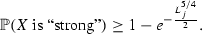
• (b) Let, for $i=1,2,\ldots L_j^{3/2}$, . Then for each $i$,

  

Proof

We only prove part (b). Part (a) is similar. Let $Y$ be a fixed semi-bad block at level $j$. Each of the events $\{X_k\hookrightarrow Y\}$ are independent, they are independent conditional on $\mathcal E _i$ as well. Now, for $k>i$

$$\begin{aligned} \mathbb P (X_k\hookrightarrow Y|\mathcal E _i)\ge 1-1/20k_0 R_{j+1}^{+} \end{aligned}$$

(63)

and for $k\le i$

$$\begin{aligned} \mathbb P (X_k\hookrightarrow Y|\mathcal E _i)\ge (1-1/20k_0 R_{j+1}^{+}-L_j^{-\delta }). \end{aligned}$$

(64)

Since $L_0$ is sufficiently large, we have $L_j^{\delta }>60 k_0 R_{j+1}^{+}$. It then follows that, conditional on $\mathcal E _i$,

$$\begin{aligned} \#\{k:X_k\hookrightarrow Y\}\succeq V \end{aligned}$$

where $V$ has a $\hbox {Bin}(\lfloor L_j^{3/2} \rfloor , (1-1/15k_0 R_{j+1}^{+}))$ distribution. Using Hoeffding’s inequality, we get

$$\begin{aligned}&\mathbb P (\#\{k:X_k\hookrightarrow Y\} \ge \lfloor L_j^{3/2} \rfloor (1-1/10k_0 R_{j+1}^{+})|\mathcal E _i)\\&\quad \ge \mathbb P (V\ge \lfloor L_j^{3/2} \rfloor (1-1/10k_0 R_{j+1}^{+})) \ge 1- 2e^{-\frac{\lfloor L_j^{3/2} \rfloor }{450k_0^2(R_{j+1}^{+})^2}} \ge 1-e^{-L_j^{5/4}} \end{aligned}$$

for $L_0$ sufficiently large. Since the length of a semi-bad block at level $j$ can be at most $10L_j$, and semi-bad blocks can contain only the first $L_j^m$ many characters, there can be at most $L_j^{10mL_j}$ many semi-bad blocks at level $j$.

Hence, using a union bound we get, for each $i$,

for large enough $L_0$, completing the proof of the lemma. $\square$

Proof of Theorem 9.1

To avoid repetition, we only prove the theorem for $\mathbb X$-blocks.

Recall the notation of Observation 3.2 with $(X_1,X_2,X_3,\ldots ..)$ a sequence of independent $\mathbb X$-blocks at level $j$ with the first $L_j^3$ conditioned to be good and $X\sim \mu _{j+1}^\mathbb{X }$ be the $(j+1)$-th level block constructed from them. Let $W_X$ be the $\hbox {Geom}(L_j^{-4})$ variable associated with $X$ and $T_X$ be the number of excess blocks. Let us define the following events.

$$\begin{aligned} A_1&= \{(X_{i},X_{i+1},\ldots X_{i+\lfloor L_j^{3/2} \rfloor }) \, \text {is a strong sequence for}~1\le i\le 2L_j^{\alpha -1}\}.\\ A_2&= \{\#\{1\le i\le L_j^{\alpha -1}+2L_j^3 + T_X: X_i \notin G_j^\mathbb{X }\}\le k_0 \}.\\ A_3&= \{\#\{1\le i\le 2L_j^{\alpha -1}: X_i \notin G_j^\mathbb{X }\cup SB_j^\mathbb{X }\}=0\}.\\ A_4&= \{T_X\le L_j^5-2L_j^3\}. \end{aligned}$$

From the definition of good blocks it follows that

$$\begin{aligned} \mathbb P (X\in G_{j+1}^\mathbb{X })\ge \mathbb P (A_1\cap A_2\cap A_3\cap A_4). \end{aligned}$$

(65)

Now, to complete the proof we need suitable estimates for the quantities $\mathbb P (A_i)$, $i=1,2,3,4$, each of which we now compute.

• Let $\tilde{X_i}=(X_{i+1},X_{i+2},\ldots ,X_{i+ \lfloor L_j^{3/2} \rfloor })$. From Lemma 9.2, it follows that for each $i$,

  

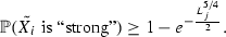
  It follows that

  $$\begin{aligned} \mathbb P [A_1^c]\le 2L_j^{\alpha -1} e^{-\frac{L_j^{5/4}}{2}}\le \frac{1}{10}L_{j+1}^{-\delta } \end{aligned}$$

  (66)

  since $L_0$ is sufficieciently large.

• By Lemma 7.3 we have that

  $$\begin{aligned} \mathbb P [A_2] \ge 1-L_j^{-\delta k_0/4}\ge 1-\frac{1}{10}L_{j+1}^{-\delta } \end{aligned}$$

  (67)

  since $k_0 >4\alpha$.

• From the definition of semi-bad blocks, we know that for $i>L_j^3$,

  $$\begin{aligned} \mathbb P (X_i \notin G_j^\mathbb{X }\cup SB_j^\mathbb{X })&\le \mathbb P \left( S_j^\mathbb{X }(X_i)\le 1-\frac{1}{20k_0 R_{j+1}^{+}}\right) + \mathbb P (|X_i|>10L_j)\\&\quad +\mathbb P (C_k\in X_i ~\text {for some}~k>L_j^m). \end{aligned}$$

Claim

We have

$$\begin{aligned} \mathbb P (C_k\in X_i ~\text {for some}~k>L_j^m)\le \mu ^\mathbb{X }(\{C_{L_j^m+1}, C_{L_j^{m}+2},\ldots \})\mathbb E (|X_i|). \end{aligned}$$

(68)

Proof of Claim

Let $A_r$ denote the event that $\{C_k\in X_r^{(j)} ~\text {for some}~k>L_j^m\}$ where $X_r^{(j)}$ denotes the $r$-th block at level $j$. Observation 3.1 and strong law of large numbers then imply

$$\begin{aligned} \lim \frac{1}{n}\sum _{r=1}^n I(A_r) = \mathbb P (C_k\in X_i ~\text {for some}~k>L_j^m)~\text {a.s.}~. \end{aligned}$$

(69)

Let $B_s$ denote the event that $\{X_s^{(0)}=C_k ~\text {for some}~k>L_j^m\}$ where $X_s^{(0)}$ denotes the $s$-th element of the sequence $\mathbb X$, i.e., the s-th block at level 0. Observe that

$$\begin{aligned} \limsup _{n\rightarrow \infty } \frac{1}{n}\sum _{r=1}^n I(A_r) \le \limsup _{N\rightarrow \infty } \frac{\sum _{s=1}^{N} I(B_s)}{\max \{t: \sum _{h=1}^t |X_h^{(j)}|\le N\}}~\text {a.s.}~. \end{aligned}$$

(70)

Dividing the numerator and denominator of the right hand side of (70) by $N$ and using strong law of large numbers again we get that the a.s. limit of the right hand side of (70) is $\mu ^\mathbb{X }(\{C_{L_j^m+1}, C_{L_j^{m}+2},\ldots \}) \mathbb E (|X_i|)$. Comparing (69) and (70) completes the proof of the claim.

Using (1) and (9), it follows that $\mathbb P (C_k\in X_i ~\text {for some}~k>L_j^m)\le 3L_j^{1-m} \le L_j^{-\beta }$ for $L_0$ large enough and since $m> 2+\beta$.

Since for $L_0$ sufficiently large, $1-\frac{1}{20k_0R_{j+1}^{+}}\le 1-L_{j}^{-1}$, using (7) and (9) we see that

$$\begin{aligned} \mathbb P (X_i \notin G_j^\mathbb{X }\cup SB_j^\mathbb{X })\le (1-\frac{1}{20k_0 R_{j+1}^{+}})^{m}L_j^{-\beta }+ \mathbb P (|X_i|>10L_j)+L_j^{-\beta }\le 3L_j^{-\beta } \end{aligned}$$

since $\alpha >6$.

Hence it follows that

$$\begin{aligned} \mathbb P [A_3^c]\le 6L_j^{\alpha -\beta -1} \le \frac{1}{10} L_{j+1}^{-\delta } \end{aligned}$$

(71)

for sufficiently large $L_0$ since $\beta > \alpha \delta +\alpha -1$.

• By Lemma 7.3 we have that

  $$\begin{aligned} \mathbb P [A_4] \ge 1-2\exp \left( -\frac{1}{4} L_j\right) \ge 1-\frac{1}{10}L_{j+1}^{-\delta }. \end{aligned}$$

  (72)

Now from (65), (66), (67), (71), (72) it follows that,

$$\begin{aligned} \mathbb P (X\in G_{j+1}^\mathbb{X })\ge 1-\sum _{i=1}^4 \mathbb P [A_i^c]\ge 1-L_{j+1}^{-\delta }, \end{aligned}$$

completing the proof of the theorem. $\square$

9.2 Mappings of good segments

Theorem 9.3

Let $\tilde{X}=(\tilde{X}_1,\tilde{X}_2,\ldots )$ be a sequence of $\mathbb X$-blocks at level $(j+1)$ and $\tilde{Y}=(Y_1,Y_2,\ldots )$ be a sequence of $\mathbb Y$-blocks at level $(j+1)$. Further we suppose that $\tilde{X}^{[1,R_{j+1}^{+}]}$ and $\tilde{Y}^{[1,R_{j+1}^{+}]}$ are “good segments”. Then for every $t$ with $R_{j+1}^{-}\le t \le R_{j+1}^{+}$,

$$\begin{aligned} \tilde{X}^{[1,R_{j+1}]}\hookrightarrow \tilde{Y}^{[1,t]}~\quad \text {and}\quad ~\tilde{X}^{[1,t]}\hookrightarrow \tilde{Y}^{[1,R_{j+1}]}. \end{aligned}$$

(73)

Proof

Let us fix $t$ with $R_{j+1}^{-}\le t \le R_{j+1}^{+}$. We only prove that $\tilde{X}^{[1,R_{j+1}]}\hookrightarrow \tilde{Y}^{[1,t]}$, the other part follows similarly.

Let $\tilde{X}^{[1,R_{j+1}]}=(X_1,X_2,\ldots ,X_n)$ be the decomposition of $\tilde{X}^{[1,R_{j+1}]}$ into level $j$ blocks. Similarly let $\tilde{Y}^{[1,t]}=(Y_1,Y_2,\ldots ,Y_{n^{\prime }})$ denote the decomposition of $\tilde{Y}^{[1,t]}$, into level $j$ blocks.

Before proceeding with the proof, we make the following useful observations. Since both $\tilde{X}^{[1,R_{j+1}]}$ and $\tilde{Y}^{[1,t]}$ are good segments, it follows that $R_{j+1}L_j^{\alpha -1}\le n \le R_{j+1}(L_j^{\alpha -1}+L_j^{5})$, and $tLj^{\alpha -1}\le n^{\prime }\le t(L_j^{\alpha -1}+L_j^{5})$. Since $L_0$ large enough and $\alpha >6$, we have

$$\begin{aligned} \frac{1-2^{-(j+7/4)}}{R}\le \frac{n^{\prime }}{n} \le R(1+2^{-(j+7/4)}). \end{aligned}$$

(74)

Let $B_X=\{1\le i \le n: X_i\notin G_j^\mathbb{X }\}=\{l_1<l_2<\cdots <l_{K_X}\}$ denote the positions of “bad” $\mathbb X$-blocks. Similarly, let $B_Y=\{1\le i \le n^{\prime }: Y_i\notin G_j^\mathbb{Y }\}=\{l^{\prime }_1<l^{\prime }_2<\cdots <l^{\prime }_{K_Y}\}$ denote the positions of “bad” $\mathbb Y$-blocks. Notice that $K_X,K_Y \le k_0R_{j+1}^{+}$. Using Proposition 6.1 we can find a family of admissible generalised mappings $\Upsilon _h$, $1\le h \le L_j^2$ which are of $Class~G^j$ with respect to $(B_X,B_Y)$, given by $\Upsilon _h([n],[n^{\prime }],B_X,B_Y)=(P_h,P^{\prime }_h,\tau _h)$ such that for all $h$, $1\le h\le L_j^2$, $1\le i\le K_X$, $1\le r \le K_Y$, $\tau _h(l_i)=\tau _{1}(l_i)+h-1$ and $\tau _h^{-1}(l^{\prime }_r)=\tau _1^{-1}(l^{\prime }_r)-h+1$. At this point we need the following lemma.

Lemma 9.4

Let $\Upsilon _h=(P_h,P^{\prime }_h,\tau _h), 1\le h\le L_j^2$ be the set of generalised mappings as described above. Then there exists $1\le h_0 \le L_j^2$, such that $X_{l_i}\hookrightarrow Y_{\tau _{h_0}(l_i)}$ for all $1\le i\le K_X$ and $X_{\tau _{h_0}^{-1}(l^{\prime }_i)}\hookrightarrow Y_{l^{\prime }_i}$ for all $1\le i \le K_Y$.

Proof

Once again we appeal to the probabilistic method. First observe that for any fixed $i$, $\{\tau _h(l_i):h=1,2,\ldots L_j^2\}$ is a set of $L_j^2$ consecutive integers. Notice that the $j$-th level sub-blocks corresponding to these indices need not belong to the same $(j+1)$-th level block. However, they can belong to at most 2 consecutive $(j+1)$-level blocks (both of which are good). Suppose the number of sub-blocks belonging to the two different blocks are $a$ and $b$, where $a+b=L_j^2$. Now, by the strong sequence assumption, these $L_j^2$ blocks the must contain at least $\lfloor \frac{a}{L_j^{3/2}}\rfloor +\lfloor \frac{b}{L_j^{3/2}}\rfloor \ge \lfloor L_j^{1/2}\rfloor -2$ many disjoint strong sequences of length $\lfloor L_j^{3/2} \rfloor$. By definition of strong sequences then, there exist, among these $L_j^2$ sub-blocks, at least $(L_j^{1/2} -3)L_j^{3/2}(1-\frac{1}{10k_0R_{j+1}^{+}})$ many to which $X_{l_i}$ can be successfully mapped, i.e.,

$$\begin{aligned} \#\{h: X_{l_i}\hookrightarrow Y_{\tau _h(l_i)}\}\ge (L_j^{1/2} -3)L_j^{3/2}\left( 1-\frac{1}{10k_0R_{j+1}^{+}}\right) . \end{aligned}$$

(75)

Now, choosing $H$ uniformly at random from $\{1,2,\ldots ,L_j^2\}$, it follows from (75) that for each $i$, $1\le i \le K_X$

$$\begin{aligned} \mathbb P (X_{l_i}\hookrightarrow Y_{\tau _H(l_i)})\ge (1-3/L_j^{1/2})\left( 1-\frac{1}{10k_0R_{j+1}^{+}}\right) \ge 1-\frac{1}{10k_0R_{j+1}^{+}}-\frac{3}{L_j^{1/2}}.\nonumber \\ \end{aligned}$$

(76)

Similar arguments show that for all $i\in \{1,2,\ldots ,K_Y\}$,

$$\begin{aligned} \mathbb P (X_{\tau _H^{-1}(l^{\prime }_i)}\hookrightarrow Y_{l^{\prime }_i})\ge 1-\frac{1}{10k_0R_{j+1}^{+}}-\frac{3}{L_j^{1/2}}. \end{aligned}$$

(77)

A union bound then gives,

$$\begin{aligned}&\mathbb P (X_{l_i}\hookrightarrow Y_{\tau _H(l_i)}: 1\le i \le K_X,~X_{\tau _H^{-1}(l^{\prime }_i)}\hookrightarrow Y_{(l^{\prime }_i)}: 1\le i \le K_Y)\ge 1\\&\quad - 2k_0R_{j+1}^{+}\left( \frac{1}{10k_0R_{j+1}^{+}}+ \frac{3}{L_j^{1/2}}\right) , \end{aligned}$$

and the right hand side is always positive for $L_0$ sufficiently large. The lemma immediately follows from this. $\square$

The proof of Theorem 9.3 can now be completed using Proposition 5.3. $\square$

9.3 Good blocks map to good blocks

Theorem 9.5

Let $X\in G_{j+1}^\mathbb{X }, Y\in G_{j+1}^\mathbb{Y }$, then $X\hookrightarrow Y$.

The theorem follows from a simplified version of the proof of Theorem 9.3 so we omit the proof.

We have now completed all the parts of the inductive step. Together these establish Theorem 4.1.

10 Explicit constructions

Our proof provides an implicit construction of a deterministic sequence $(X_1,\ldots )$ which embeds into $\mathbb Y$ with positive probability. We will describe a deterministic algorithm, based on our proof, which for any $n$ will return the first $n$ co-ordinates of the sequence in finite time. Though it is not strictly necessary, we will restrict discussion to the case of finite alphabets. It can easily be seen from our construction and proof that any good $j$-level block can be extended into a $(j+1)$-level good block and so the algorithm proceeds by extending one good block to one of the next level. As such one only needs to show that we can identify all the good blocks at level $j$ in a finite amount of time.

We will also recover all semi-bad blocks. By our construction all good and semi-bad blocks are of bounded length so there is only a finite space to examine. To determine if a block is good at level $j+1$ one needs to count how many of its sub-blocks at level $j$ are good and verify that the others are semi-bad. It also requires that it has “strong subsequences”. This can be computed if we have a complete list of semi-bad $j$-level blocks.

Determining if $X$, a $(j+1)$-level block, is semi-bad requires calculating its length and its embedding probability. For this we need to run over all possible $(j+1)$-level blocks, calculate their probability and then test if $X$ maps into them. By the definition of an $R$-embedding we need only consider those of length at most $O(R |X|)$ so this can be done in finite time.

With this listing of all good blocks one can then construct in an arbitrary manner a sequence in which the first block is good at all levels which will have a positive probability of an $R$-embedding into a random sequence. From this construction, and the reduction in § 2, we can construct a deterministic sequences which has an $M$-Lipshitz embedding into a random binary sequence in the sense of Theorem 1 with positive probability. Similarly, this approach gives a binary sequence with a positive density of ones which is compatible sequence with a random $\hbox {Ber}(q)$ sequence in the sense of Theorem 3 for small enough $q>0$ with positive probability.

References

Abért, M.: Asymptotic group theory questions. Available at http://www.math.uchicago.edu/~abert/research/asymptotic.html (2008)
Balister, P.N., Bollobás, B., Stacey, A.M.: Dependent percolation in two dimensions. Probab. Theory Relat. Fields 117, 495–513 (2000)
Benjamini, I., Kesten, H.: Percolation of arbitrary words in \(\{0,1\}^{ N}\). Ann. Probab. 23(3), 1024–1060 (1995)
Coppersmith, D., Tetali, P., Winkler, P.: Collisions among random walks on a graph. SIAM J. Discrete Math. 6, 363 (1993)
de Lima, B.N.B., Sanchis, R., Silva, R.W.C.: Percolation of words on \(\mathbb{Z}^d\) with long-range connections. J. Appl. Probab. 48(4), 1152–1162 (2011)
Dirr, N., Dondl, P.W., Grimmett, G.R., Holroyd, A.E., Scheutzow, M.: Lipschitz percolation. Electron. Comm. Probab. 15, 14–21 (2010)
Gács, P.: Compatible sequences and a slow Winkler percolation. Combin. Probab. Comput. 13(6), 815–856 (2004)
Gács, P.: Clairvoyant scheduling of random walks. Random Str. Algorithm 39, 413–485 (2011)
Gács, P.: Clairvoyant embedding in one dimension. Preprint (2012)
Grimmett, G.: Three problems for the clairvoyant demon. Arxiv, preprint arXiv:0903.4749 (2009)
Grimmett, G.R., Holroyd, A.E.: Geometry of lipschitz percolation. Ann. Inst. H. Poincaré Probab. Statist. 48(2), 309–326 (2012)
Grimmett, G.R., Holroyd, A.E.: Plaquettes, spheres, and entanglement. Electr. J. Probab. 15, 1415–1428 (2010)
Grimmett, G.R., Holroyd, A.E.: Lattice embeddings in percolation. Ann Probab. 40(1), 146–161 (2012)
Grimmett, G.R., Liggett, T.M., Richthammer, T.: Percolation of arbitrary words in one dimension. Random Str. Algorithm 37(1), 85–99 (2010)
Gromov, M.: Hyperbolic manifolds, groups and actions. In: Proceedings of the 1978 Stony Brook Conference, Riemann Surfaces and Related Topics, pp. 183–213 (1981)
Holroyd, A.E., Martin, J.: Stochastic domination and comb percolation. Arxiv, preprint arXiv: 1201.6373 (2012)
Kanai, M.: Rough isometries, and combinatorial approximations of geometries of non. compact riemannian manifolds. J. Math. Soc. Jpn. 37(3), 391–413 (1985)
Kesten, H., de Lima, B., Sidoravicius, V., Vares. M.E.: On the compatibility of binary sequences. Preprint arXiv:1204.3197 (2012)
Kesten, H., Sidoravicius, V., Vares, M.E.: Percolation in dependent environment. Preprint (2012)
Kesten, H., Sidoravicius, V., Zhang, Y.: Almost all words are seen in critical site percolation on the triangular lattice. Elec. J. Probab. 3, 1–75 (1998)
Kesten, H., Sidoravicius, V., Zhang, Y.: Percolation of arbitrary words on the close-packed graph of \(\mathbb{Z}^2\). Electr. J. Probab. (electronic) 6, 4–27 (2001)
Peled, R.: On rough isometries of poisson processes on the line. Ann. Appl. Probab. 20, 462–494 (2010)
Sidoravicius, V.: Percolation of binary words and quasi isometries of one-dimensional random systems. Preprint (2012)
Winkler, P.: Dependent percolation and colliding random walks. Random Str. Algorithm 16(1), 58–84 (2000)
Acknowledgments
We would like to thank Vladas Sidoravicius for describing his work on these problems and Peter Gács for informing us of his new results. We would also like to thank Geoffrey Grimmett and Ron Peled for introducing us to the Lipschitz embedding and rough isometry problems and to Peter Winkler for very useful discussions. We are grateful to an anonymous Referee for extremely careful reading of the manuscript and for many useful comments and suggestions.
Author information
Authors and Affiliations
Corresponding author
Additional information
R. Basu was supported by Loéve Fellowship, Department of Statistics, University of California, Berkeley. A. Sly was supported by NSF grant DMS-1208338 and a Sloan Fellowship.
Rights and permissions
About this article
Cite this article
Basu, R., Sly, A. Lipschitz embeddings of random sequences. Probab. Theory Relat. Fields 159, 721–775 (2014). https://doi.org/10.1007/s00440-013-0519-7
Received:
Published:
Issue Date:
DOI: https://doi.org/10.1007/s00440-013-0519-7