Unsupervised Learning

Abstract

Thus far, we have considered Supervised learning from N observation data $(x_1, y_1), \ldots , (x_N, y_N)$, where $y_1, \ldots , y_N$ take either real values (regression) or a finite number of values (classification). In this chapter, we consider unsupervised learning, in which such a teacher does not exist, and the relations between the N samples and between the p variables are learned only from covariates $x_1, \ldots , x_N$. There are various types of unsupervised learning; in this chapter, we focus on clustering and principal component analysis. Clustering means dividing the samples $x_1, \ldots , x_N$ into several groups (clusters). We consider K-means clustering, which requires us to give the number of clusters K in advance, and hierarchical clustering, which does not need such information. We also consider principal component analysis (PCA), a data analysis method that is often used for machine learning and multivariate analysis. For PCA, we consider another equivalent definition along with its mathematical meaning.

Appendices

Appendix: Program

A program that generates the dendrogram of Hierarchical clustering. After obtaining the cluster object via the function hc, we compare the distances between consecutive clusters using the ordered sample y. Specifically, we express the positions of the branches by z[k, 1], z[k, 2], z[k, 3], z[k, 4], z[k, 5].

Exercises 88–100

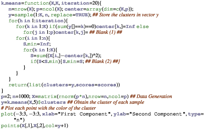
• 88. The following procedure divides N samples with p variables into K disjoint sets, given K (K-means clustering). We repeat the following two steps after randomly assigning one of $1,\ldots ,K$ to each sample.

  • (a) Compute the centers of clusters $k=1,\ldots ,K$.

  • (b) To each of the N samples, assign the nearest center among the K clusters.

  Fill in the blanks and execute the procedure.

  

• 89. The clusters that K-means clustering generates depend on the randomly chosen initial values. Repeat ten times to find the sequence of values immediately after the 2-step update. Display each transition as a line graph on the same graph.

• 90. K-means clustering minimizes

  $$S:=\sum _{k=1}^K\frac{1}{|C_k|}\sum _{i\in C_k}\sum _{i'\in C_k}\sum _{j=1}^p(x_{i,j}-x_{i',j})^2$$

  w.r.t. $C_1,\ldots ,C_K$ from data $X=(x_{i,j})$

  • (a) Show the following equation:

    $$\frac{1}{|C_k|}\sum _{i\in C_k}\sum _{i'\in C_k}\sum _{j=1}^p(x_{i,j}-x_{i',j})^2=2\sum _{i\in C_k}\sum _{j=1}^p(x_{i,j}-\bar{x}_{k,j})^2$$

    .

  • (b) Show that the score S is monotonously decreasing each time the two steps are executed in Problem 88.

  • (c) Let $N=3$, $p=1$, and $K=2$, and assume that the samples are in 0, 6, 10. We consider two cases: one and two are assigned to 0, 6 and 10, respectively; and one and two are assigned to 0 and 6, 10, respectively. What values do they converge to if the initial state is each of the two cases? What score do they finally obtain?

• 91. Write R codes for the functions dist.complete, single.complete, dist.centroid, dist.average to find the maximum distance between the rows in x, y, the minimum distance between the rows in x, y, the distance between the centers of x, y, and the average distance between the rows in x, y, given matrices x, y composed of multiple rows extracted from $X\in {\mathbb R}^{N\times p}$.

• 92. The following procedure executes hierarchical clustering w.r.t. data $x_1,\ldots ,x_N \in {\mathbb R}^p$. Initially, each cluster contains exactly one sample. We merge the clusters to obtain a clustering with any number K of clusters. Fill in the blanks and execute the procedure.

  

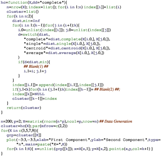
• 93. In hierarchical clustering, if we use centroid linkage, which connects the clusters with the smallest value of dist.centroid, inversion may occur, i.e., clusters with a smaller distance can be connected later. Explain the phenomenon for the case (0, 0), (5, 8), (9, 0) with $N=3$ and $p=2$.

• 94. Let $\Sigma =X^TX/N$ for $X\in {\mathbb R}^{N\times p}$, and let $\lambda _i$ be the i-th largest eigenvalue in $\Sigma$.

  • (a) Show that the $\phi$ that maximizes $\Vert X\phi \Vert ^2$ among $\phi \in {\mathbb R}^N$ with $\Vert \phi \Vert =1$ satisfies $\Sigma \phi =\lambda _1\phi$.

  • (b) Show $\phi _1,\ldots ,\phi _m$ such that $\Sigma \phi _1=\lambda _1\phi _1,\ldots ,$ $\Sigma \phi _m=\lambda _m\phi _m$ are orthogonal when $\lambda _1>\cdots >\lambda _m$.

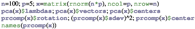
• 95. Using the eigen function in the R language, write an R program pca that outputs the average of the p columns, the eigenvalues $\lambda _1,\ldots ,\lambda _p$, and the matrix that consists of $\phi _1,\ldots ,\phi _p$ by specifying pca(X)$centers, pca(X)$lambdas, and pca(X)$vectors, respectively, given input $X\in {\mathbb R}^{N\times p}$. Moreover, execute the following to show that the results obtained via pca and prcomp coincide.

  

• 96. The following procedure produces the first and second principal component vectors $\phi _1$ and $\phi _2$ from N samples $(x_1,y_1),\ldots ,(x_N,y_N)$. Fill in the blanks, and execute it.

  

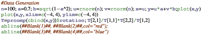
  Moreover, show that the product of the slopes is $-1$.

• 97. There is another equivalent definition of PCA. Suppose that we have centralized the matrix $X\in {\mathbb R}^{N\times p}$, and let $x_i$ be the i-th row vector of $X\in {\mathbb R}^{N\times p}$ and $\Phi \in {\mathbb R}^{p\times m}$ be the matrix that consists of the mutually orthogonal vectors $\phi _1,\ldots ,\phi _m$ of unit length. Then, we can obtain the projection $z_1=x_1\Phi ,\ldots ,z_N=x_N\Phi \in {\mathbb R}^m$ of $x_1,\ldots ,x_N$ on $\phi _1,\ldots ,\phi _m$. We evaluate how the $x_1,\ldots ,x_N$ are recovered by $L:=\sum _{i=1}^N \Vert x_i-x_i\Phi \Phi ^T\Vert ^2$, which is obtained by multiplying $z_1,\ldots ,z_N$ by $\Phi ^T$ from the right. We can regard PCA as the problem of finding $\phi _1,\ldots ,\phi _m$ that minimize the value. Show the two equations.

  $$\begin{aligned}&\displaystyle \sum _{i=1}^N\Vert x_i-x_i\Phi \Phi ^T\Vert ^2=\sum _{i=1}^N\Vert x_i\Vert ^2-\sum _{i=1}^N\Vert x_i\Phi \Vert ^2 \\&\displaystyle \sum _{i=1}^N\Vert x_i\Phi \Vert ^2=\sum _{j=1}^m\Vert X \phi _j\Vert ^2. \end{aligned}$$

• 98. We prepare a data set containing the numbers of arrests for four crimes in all fifty states.

  

  • (a) Look up the attributes via names(pr.out) and display the result.

  • (b) Execute biplot(pr.out), multiply the values of pr.out$x and pr.out$rotation by $-1$, and execute biplot(pr.out).

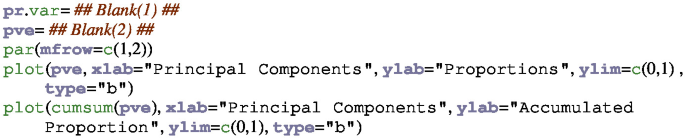
• 99. The proportions and accumulated proportion are defined by $\displaystyle \frac{\lambda _k}{\sum _{j=1}^p\lambda _j}$ and $\displaystyle \frac{\sum _{k=1}^m\lambda _k}{\sum _{j=1}^p\lambda _j}$ for each $1\le m\le p$. Fill in the blanks and draw the graph.

  

• 100. In addition to PCA and linear regression, we may use principal component regression: find the matrix $Z=X\Phi \in {\mathbb R}^{N\times m}$ that consists of the m principal components obtained via PCA, find $\theta \in {\mathbb R}^m$ that minimizes $\Vert y-Z\theta \Vert ^2$, and display via $\hat{\theta }$ the relation between the response and m components (a replacement of the p covariates). Principal component regression regresses y on the columns of Z instead of those of X.

  Show that $\Phi \hat{\theta }$ and $\beta =(X^TX)^{-1}X^Ty$ coincide for $m=p$. Moreover, fill in the blanks and execute it.

  

  Hint: Because $\min _\beta \Vert y-X\beta \Vert ^2\le \min _\theta \Vert y-X\Phi \theta \Vert ^2=\min _\theta \Vert y-Z\theta \Vert ^2$, it is sufficient to show that there exists $\theta$ such that $\beta =\Phi \theta$ for an arbitrary $\beta \in {\mathbb R}^p$ when $p=m$.