
Abstract
We discuss a new method of how the (nonlinear) 2D shallow water fluid dynamic problems inspired by ocean hydraulics, meteorology etc. can be modeled by internally passive multidimensional Kirchhoff circuits which subsequently pave the way for robust numerical simulation of the system by wave digital techniques. While the specific fluid dynamic equations dealt with in this paper are important in their own right and can be used to model a number of physical phenomena, the treatment is only one of many examples of the basic tenet that it should be possible to model all properly described physical systems by multidimensional internally passive Kirchhoff circuits. We refer to this as the Kirchhoff paradigm. In the context of the present specific problem, the paper thus helps to bridge connections between physics and circuits and systems theory at a deeper level than has been exploited before.


Notes
The 3D shallow water theory (Vreugdenhil 1994), not consider here, allows \(\uprho \) to be a function of \(z\), but the boundary conditions discussed next at the top and bottom surface of the fluid remain in force.
See Appendix 2 for a compact version using vector-matrix notation.
Terms related in this way are equivalent from the point of view of the dynamics of perturbations.
Here, with a slight abuse of notation we use the symbols \(\upalpha \) and \(\upbeta \) to denote the parameters of the differential adaptor, and they have nothing to do with the variables \(\upalpha \) and \(\upbeta \) used in Sects. 3 and 4 of this text.
Fig. 8 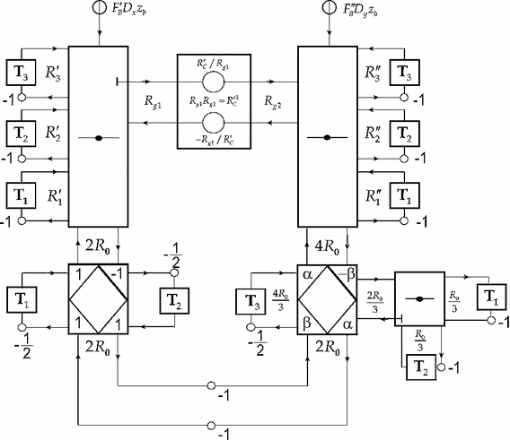
Wave digital realization of MD Kirchhoff circuit in Fig. 7
Note that the corresponding quantity in gas dynamics turns out to be the velocity of sound \(v_s\). The ratio of flow velocity with \(v_w\) is called the Froude number, and plays the role of aerodynamic Mach number. A flow is considered supercritical if the flow velocity is larger than \(v_w =\sqrt{ga}\), and subcritical otherwise (as for supersonic or subsonic flows in aerodynamics).

References
Bilbao, S. (2004). Wave and scattering methods for numerical simulation. New York: Wiley.
Fettweis, A. (1986). Wave digital filters: Theory and practice. Proceedings of the IEEE, 74(2), 270–327.
Fettweis, A., & Nitsche, G. (1991a). Numerical integration of partial differential equations using principles of multidimensional wave digital filters. In J. A. Nossek (Ed.), Parallel processing on VLSI arrays (pp. 7–24). Boston, MA: Kluwer Academic Publishers.
Fettweis, A., & Nitsche, G. (1991b). Transformation approach to numerically integrating PDE’s by means of WDF principles. Multidimensional Systems and Signal Processing, 2, 127–159.
Fettweis, A. (1992). Discrete modeling of lossless fluid dynamic systems. Archiv für Elektronik und Übertragungstechnik, 46(4), 209–218.
Fettweis, A. (2002). Improved wave digital approach to numerically integrating the PDEs of fluid dynamics. Proceedings of the ISCAS, III, 361–364.
Fettweis, A. (2006). Robust numerical integration using wave-digital concepts. Multidimensional Systems and Signal Processing, 17(1), 7–25.
Fettweis, A., & Basu, S. (2011). Multidimensional causality and passivity of linear and nonlinear systems arising from physics. Multidimensional Systems & Signal Processing, 22, 5–25.
Fjordholma, U. S., Mishra, S., & Tadmor, E. (2011). Well-balanced and energy stable schemes for the shallow water equations with discontinuous topography. Journal of Computational Physics, 230, 5587–5609.
Kundu, P. K., Cohen, I. M., & Dowling, D. R. (2012). Fluid mechanics (5th ed.). New York: Academic Press (Elsevier publications).
Petersen, D. P., & Middleton, D. (1962). Sampling and reconstruction of wave-number-limited functions in N-dimensional Euclidean spaces. Information and Control, 5, 279–323.
Tadmor, E., & Zhong, W. (2008). Energy-preserving and stable approximations for the two-dimensional shallow water equations. In H. Munthe-Kaas & B. Owren (Eds.), Mathematics and computation—A contemporary view, Proceedings of the third Abel Symposium (pp. 67–94). Springer.
Tan, W. Y. (1992). Shallow water hydrodynamics: Mathematical theory and numerical solution for a two-dimensional system of shallow-water equations. London: Elsevier Publications.
Tseng, C. H. (2012). Modeling and visualization of a time-dependent shallow water system using nonlinear Kirchhoff circuit. IEEE Transactions on Circuits and Systems Part-I, 59(6), 1265–1277.
Tseng, C. H. (2013). Numerical stability verification of a two-dimensional time-dependent nonlinear shallow water system using multidimensional wave digital filtering network. Circuits Systems & Signal Processing, 32, 299–319.
Vreugdenhil, C. B. (1994). Numerical methods for shallow-water flow. Berlin: Springer.
Whitham, G. B. (1974). Linear and nonlinear waves. New York: Wiley.
Acknowledgments
The authors would like to thank the anonymous reviewers for suggesting several improvements to the exposition of the present paper, which have been addressed in preparing the present version to the extent possible.
Author information
Authors and Affiliations
Corresponding author
Appendices
Appendix 1
1.1 Appendix 1.1: Rule for combining nonlinear inductances
A nonlinear inductance with an intro (current-like) variable \(i\) flowing through it and with an ultro (voltage-like) variable \(u\) across it is defined by the relation
where all three expressions given for the ultro \(u\) are indeed equivalent. Interestingly, it is easy to see that if we have two relations of the above form involving the same \(i\), i.e.,
then we also have
One might note that the expression for \(u_1 \pm u_2\) in the above formula can be interpreted as nonlinear extensions of well-known formula for combining constant valued inductances in series.
1.2 Appendix 1.2: Compact representation of 2D shallow water equations
The set of three 2D shallow water Eqs. (4.1) can be written in a compact form as in:
where \(\nabla _H \equiv (D_x,D_y )^{T}\) is the 2D gradient operator, \(D_S \equiv D_t +\mathbf{v}^{T}\nabla _H \) is the material derivative in the 2D shallow water context, \(\mathbf{S}\) is the skew anti-symmetric matrix \(\mathbf{S}=\left[ \begin{array}{r@{\quad }l} 0&{}1\\ -1&{}0\\ \end{array}\right] \), and as usual \(\mathbf{v}=(\bar{{v}}_x ,\bar{{v}}_y )^{T}\).
Appendix 2: Adaptor configuration associated with differential transformers
We have extensively made use of special cases of the four-port differential transformers configuration shown in Fig. 9a. We assume the eight terminals be paired into the four ports 1 to 4 characterized by the four ultro-intro pairs \((u_1,i_1 )\) to \((u_4 ,i_4 )\). Under the assumption that the port conditions are satisfied at all the four ports of the circuit in Fig. 9, they are described by the equations
Denoting the power waves by \(a_\upnu \) and \(b_\upnu \), we have
Using standard vector-matrix notation we can write
where \(\mathbf{S}\) is the (power wave) scattering matrix associated with the four-port differential transformer. The matrix \(\mathbf{S}\) can be determined by eliminating \(u_1\) to \(u_4\) and \(i_1\) to \(i_4 \) between (7.2)–(7.4). If the port resistances satisfy
one finds the simple relations
The matrix \(\mathbf{S}\) describes the (power wave) differential adaptor. The block representation of the corresponding differential adaptor is shown in Fig. 9b. The adaptor block comprises an inscribed diamond whose edges indicate the coupling between the ports. One of these edges is shown with bold faced line and three others by thin lines, the former corresponding to a negative coefficients and the others to positive coefficients.

Four-port differential transformer and its corresponding differential adaptor
For example, the output at port 2 is dependent on the input at port 4 via a coefficient \(\upalpha \) and on the input at port 3 via \(-\upbeta \), altogether thus such that \(b_2 =-\upbeta a_3 +\upalpha a_4\), as can indeed be verified from (7.5) and (7.7). The output at any port is independent of the input at the same port and also of the input at the port across the diamond, thus ensuring that all four ports are reflection free, and furthermore the pairs of ports facing each other are mutually decoupled.
A detailed flow diagrams is shown in Fig. 10a. The pair of multipliers \(\upalpha \) in the \(b_3 \)-branch and in the \(a_3 \)-branch can frequently be merged with into a single multiplier of value \(\upalpha ^{2}=1/(m+1)\). In particular, as shown in Fig. 10b, if elements such as an inductance, a capacitance, or a resistance are connected to ports 3 and 4, no delay free path will be created from input to output, neither at port 1 nor at port 2. This assumes of course that the requirements (7.6) can indeed be satisfied, but this turns out to be frequently the case in practical applications as e.g., in the present paper. Further simplification is possible if \(m=1\) because the multiplier \(\upalpha ^{2}=1/2\), can then be implemented without any true floating point multiplication in hardware realization. This possibility is shown in Fig. 10c and has indeed been used with the differential transformers in Figs. 5 and 6.

a Signal-flow diagram of differential adaptor (cf. Fig. 9b) with terminations in relevant shift vectors \(\mathbf{{T}'}\) and \(\mathbf{{T}''}\); b with pairs of \(\upalpha \)-multipliers combined; c further simplification when \(m=1\)
Appendix 3: Constrained adaptors with a source
While power wave adaptors were indeed described in (Fettweis 1986, Section IX-H, pp. 311–312), for the convenience of the reader we repeat such considerations including series interconnections involving ultro sources. We consider a series connection of an ultro source \(u_s\) and \(n\) ports with \(u_\upnu ,\,\upnu =1\) to \(n\) being the ultro variables at the ports. In the context of this paper we have \(n=5\). By definition of series connection we have
where \(i\) is the common intro variable. We then have for each \(\upnu =1\) to \(n\) the incident and reflected power waves as
where \(R_\upnu >0\) denotes the port resistances. Eliminating \(u_\upnu \) and \(i_\upnu ,\,\upnu =1\;\hbox {to }n\) we obtain the power waves quantities, again for \(\upnu =1\;\hbox {to }n\)
These results differ from those for standard adaptors (Fettweis 1986) only by the terms in \(u_s\) and \(a_s\). As for standard adaptors, if an ultro source is present, one can still make one of the ports reflection-free, e.g., by having
and consequently, with \(a_0 = \upgamma _1 a_1 + \mathrm{L} + \upgamma _{n-1} a_{n-1},\)
The corresponding adaptors are as used in Figs. 6 and 8 with \(n=5\).
Rights and permissions
About this article

Cite this article
Basu, S., Fettweis, A. A new look at 2D shallow water equations of fluid dynamics via multidimensional Kirchhoff paradigm. Multidim Syst Sign Process 26, 1001–1034 (2015). https://doi.org/10.1007/s11045-015-0321-z
Received:
Revised:
Accepted:
Published:
Issue Date:
DOI: https://doi.org/10.1007/s11045-015-0321-z