Capturing the Dynamics of a Hybrid Multiscale Cancer Model with a Continuum Model

Abstract

Cancer is a complex disease involving processes at spatial scales from subcellular, like cell signalling, to tissue scale, such as vascular network formation. A number of multiscale models have been developed to study the dynamics that emerge from the coupling between the intracellular, cellular and tissue scales. Here, we develop a continuum partial differential equation model to capture the dynamics of a particular multiscale model (a hybrid cellular automaton with discrete cells, diffusible factors and an explicit vascular network). The purpose is to test under which circumstances such a continuum model gives equivalent predictions to the original multiscale model, in the knowledge that the system details are known, and differences in model results can be explained in terms of model features (rather than unknown experimental confounding factors). The continuum model qualitatively replicates the dynamics from the multiscale model, with certain discrepancies observed owing to the differences in the modelling of certain processes. The continuum model admits travelling wave solutions for normal tissue growth and tumour invasion, with similar behaviour observed in the multiscale model. However, the continuum model enables us to analyse the spatially homogeneous steady states of the system, and hence to analyse these waves in more detail. We show that the tumour microenvironmental effects from the multiscale model mean that tumour invasion exhibits a so-called pushed wave when the carrying capacity for tumour cell proliferation is less than the total cell density at the tumour wave front. These pushed waves of tumour invasion propagate by triggering apoptosis of normal cells at the wave front. Otherwise, numerical evidence suggests that the wave speed can be predicted from linear analysis about the normal tissue steady state.

Appendices

Appendix A Parameter Values

In the multiscale model by Owen et al. (2011), a lattice site corresponds to a cube with length of each side equal to ${\varDelta }x=40\mu \text {m}=0.04\text { mm}$. Let us denote the volume of one lattice site by $V_{site}=6.4\times 10^{-5}\text { mm}^3$. For the remainder of this section, lattice site has the same meaning as above unless stated otherwise.

1.1 Estimation of $P_{c}$

We ran simulations of the multiscale model for different vessel densities on a $1\times 1$ square lattice with only one normal cell. The simulations were run only for one time step, and the oxygen concentration was noted. Since the lattice dimensions are $1\times 1$, we can assume that the system is spatially homogeneous and thus obtain $P_{c}$ by substituting the values of n, b and C in Eq. (16). The value is given in Table 3.

1.2 Estimation of $k^{cell}_{c}$, $k^{cell}_{v}$

In the multiscale model, for one cell in one lattice site, the rate of oxygen consumption by cell type cell, $k^{cell}_{c}$ $\text {min}^{-1}$, represents the rate of consumption for one cell per $V_{site}$.

Therefore, to obtain the rate in units of per cell density per min (${(\text {cell}/\text {mm}^{3})}^{-1} \text {min}^{-1}$), suitable for the continuum model, we multiply $k^{cell}_{c}$ by $V_{site}$.

The rate of VEGF secretion by cell type cell, $k^{cell}_{v}$, is also obtained similarly. The values used in the continuum model are given in Table 2.

Table 2 Parameters in the continuum model, Eqs. (13), (14), (16), (17), (19) and (21), that are modified from those of the multiscale model (Owen et al. 2011) and are related to cell proliferation (sprouting for tip cells), apoptosis, cell quiescence, oxygen consumption and VEGF secretion

1.3 Estimation of $d_{cell}$

In the multiscale model, the carrying capacity of a cell at lattice site x is defined as the maximum number of cells that can be present at x. Therefore, we obtain the carrying capacity for the continuum model as number of cells per unit volume ($\text {cells}/\text {mm}^3$) by dividing the carrying capacity by $V_{site}$. The value is given in Table 2.

Table 3 Parameters for oxygen and VEGF

Table 4 Parameters in the continuum model, Eqs. (13), (14), (16), (17), (19) and (21), that can be taken or derived directly from the multiscale model (Owen et al. 2011) and are related to cell proliferation (sprouting for tip cells), apoptosis, movement, oxygen consumption and VEGF secretion

1.4 Estimation of $D_{cell}$

In the multiscale model, apart from random movement, normal and tumour cells also spread by via cell division by placing their daughter cells in neighbouring sites if the number of cells in the parent cell’s site exceeds its carrying capacity. A cell of type cell takes at least $T_{min}^{cell}$ minutes to divide. On division, the new cell is placed in one of Moore neighbourhood sites. Thus, the mean squared displacement of the cell in $T_{min}^{cell}$ min is of the order of ${\varDelta }x$ mm.

For normal cells, the random motility coefficient, in the multiscale model, is zero. We thus estimate the value of $D_{norm}$ using the mean squared displacement estimated above. For tumour cells, the random motility coefficient in the multiscale model is non-zero. Thus, starting with the estimate obtained from the mean squared displacement of tumour cells, we simulate the continuum model for different values of $D_{tum}$ and compare the distance covered in unit time with the simulation from the multiscale model. The best fit thus obtained was chosen as the value for $D_{tum}$.

All the values of $D_{cell}$ are given in Table 4.

1.5 Estimation of $p_{1}$

In all simulations of the multiscale model presented in this paper, all vessels have a fixed radius $R = 0.006 \text { mm}$ and typical length $L={\varDelta }x$. Also, in the multiscale model, all blood vessels in a lattice site are associated with one endothelial cell. Therefore, in a lattice site with volume $V_{site}$, each vessel with surface density of $2\pi R {\varDelta }x/V_{site}=23.56\text { mm}^{2}/\text {mm}^{3}$ has an endothelial cell density of $1/V_{site}=15{,}625\text { cells}/\text {mm}^3$ associated with it. Therefore, $p_{1}$, defined as the number of endothelial cells per unit vascular surface area is obtained by dividing the endothelial cell density by the vessel surface density. Thus $p_{1}=663$ cells/mm$^2$, as given in Table 5.

Table 5 Other parameters of the continuum model

1.6 Estimation of $\lambda _{2}$

Estimating the rates of tip-tip and tip-vessel anastomosis from the multiscale model is difficult. We thus use the values given in Schnepf et al. (2008). To convert $\overline{\lambda _2}$ from units of per unit capillary length density per unit time to the units of per unit capillary surface density per unit time, we multiply $\overline{\lambda _{2}}$ from Schnepf et al. (2008) with the surface area of a vessel with radius $0.006\text { mm}$ and unit length. The values of $\lambda _1$ and $\lambda _2$ are given in Table 5.

Appendix B Normal Vasculature Tissue Model

Oxygen

$$\begin{aligned} 0 =&\;\underbrace{D_{c}\nabla ^2 C}_\text {diffusion}+\underbrace{P_{c}b(C_{blood}-C)}_\text {delivery from blood}-\underbrace{k^{norm}_{c}nC}_{\begin{array}{c} \text {consumption by}\\ \text {normal cells} \end{array}}-\underbrace{k^{vessel}_{c}(p_{1}b)C}_{\begin{array}{c} \text {consumption by}\\ \text {vessel cells} \end{array}}-\underbrace{k^{tip}_{c}(e+m)C}_{\begin{array}{c} \text {consumption by}\\ \text {tip cells} \end{array}}, \end{aligned}$$

(32a)

VEGF

$$\begin{aligned} 0 =&\; \underbrace{D_{v}\nabla ^2 V}_\text {diffusion}+\underbrace{P_{v}b(V_{blood}-V)}_\text {delivery from blood}+\underbrace{\mathscr {H}(C_{v}^{norm}-C,\epsilon _{v})k_{v}^{norm}n}_\text {secretion by normal cells}-\underbrace{\delta _{v}V}_\text {decay}, \end{aligned}$$

(32b)

Normal Cell Density

$$\begin{aligned} \frac{\partial n}{\partial t} =&\;\underbrace{D_{norm}\nabla ^2 n}_{\begin{array}{c} \text {random}\\ \text {motility} \end{array}}+\underbrace{\frac{\ln (2)}{T_{min}^{norm}}\frac{C}{C_{\phi }^{norm}+C}\mathscr {H}(d_{norm}-S_{tot},\epsilon _{d})n}_\text {proliferation}\nonumber \\&\quad -\underbrace{\mathscr {H}(C_{a}^{norm}-C,\epsilon _{a})\beta _{norm}n}_{\text {apoptosis}}, \end{aligned}$$

(32c)

Immature Tip Cell Density

$$\begin{aligned} \frac{\partial e}{\partial t} =&\;\underbrace{D_{e}\nabla ^2 e}_{\begin{array}{c} \text {random}\\ \text {motility} \end{array}}-\underbrace{\chi _{e}\nabla \Big [\Big (1-\dfrac{S_{tot}}{d_{tip}}\Big )\mathscr {S}(d_{tip}-S_{tot})e\nabla V\Big ]}_{\begin{array}{c} \text {chemotactic response in the direction}\\ \text {of increasing VEGF} \end{array}} \nonumber \\&+\underbrace{ P^{max}_{sprout}\frac{V}{V_{sprout}+V}\mathscr {H}(d_{tip}-S_{tot},\epsilon _{d})(p_{1}b)}_{\begin{array}{c} \text {generation}\\ \text {of new tips} \end{array}}\;\!-\;\!\underbrace{\alpha _{1}e}_{\begin{array}{c} \text {conversion}\\ \text {to mature}\\ \text {tip cells} \end{array}}, \end{aligned}$$

(32d)

Mature Tip Cell Density

$$\begin{aligned} \frac{\partial m}{\partial t} =&\; \underbrace{D_{e}\nabla ^2 m}_{\begin{array}{c} \text {random}\\ \text {motility} \end{array}} -\underbrace{\chi _{e}\nabla \Big [\Big (1-\dfrac{S_{tot}}{d_{tip}}\Big )\mathscr {S}(d_{tip}-S_{tot})m\nabla V\Big ]}_{\begin{array}{c} \text {chemotactic response in the direction}\\ \text {of increasing VEGF} \end{array}}+\underbrace{\alpha _{1}e}_{\begin{array}{c} \text {conversion}\\ \text {from immature}\\ \text {tip cells} \end{array}}\nonumber \\&\quad -\underbrace{\lambda _{1}m^2}_{\begin{array}{c} \text {tip-tip}\\ \text {anastomosis} \end{array}}-\underbrace{\lambda _{2}mb}_{\begin{array}{c} \text {tip-capillary}\\ \text {anastomosis} \end{array}}, \end{aligned}$$

(32e)

Blood Vessel Density

$$\begin{aligned} \frac{\partial b}{\partial t} =&\; \underbrace{\frac{1}{p_{1}}\;(\lambda _{1}m^2+\lambda _{2}mb)}_{\begin{array}{c} \text {tip-tip and tip-capillary}\\ \text {anastomosis} \end{array}}. \end{aligned}$$

(32f)

Appendix C Steady State Analysis

Assuming all the variables to be spatially homogeneous, we obtain the following set of differential algebraic equations (DAEs),

$$\begin{aligned} 0 =&\; \underbrace{P_{c}b(C_{blood}-C)}_\text {delivery from blood}- \underbrace{k^{norm}_{c}nC}_{\begin{array}{c} \text {consumption by}\\ \text {normal cells} \end{array}}-\underbrace{k^{vessel}_{c}(p_{1}b)C}_{\begin{array}{c} \text {consumption by}\\ \text {vessel cells} \end{array}}-\underbrace{k^{tip}_{c}(e+m)C}_{\begin{array}{c} \text {consumption by}\\ \text {tip cells} \end{array}},&\end{aligned}$$

(33a)

$$\begin{aligned} 0 =&\;\underbrace{P_{v}b(V_{blood}-V)}_\text {delivery from blood}- \underbrace{\mathscr {H}(C_{v}^{norm}-C,\epsilon _{v})k_{v}^{norm}n}_\text {secretion by normal cells}-\underbrace{\delta _{v}V}_\text {decay},&\end{aligned}$$

(33b)

$$\begin{aligned} \dfrac{\hbox {d}n}{\hbox {d}t} =&\; \underbrace{\dfrac{\ln (2)}{T_{min}^{norm}}\dfrac{C}{C_{\phi }^{norm}+C}\mathscr {H}(d_{norm}-S_{tot},\epsilon _{d})n}_\text {proliferation}-\underbrace{\mathscr {H}(C_{a}^{norm}-C,\epsilon _{a})\beta _{norm}n}_{\text {apoptosis}},&\end{aligned}$$

(33c)

$$\begin{aligned} \dfrac{\hbox {d}e}{\hbox {d}t} =&\; \underbrace{P^{max}_{sprout}\dfrac{V}{{V_{sprout}+V}}\mathscr {H}(d_{tip}-S_{tot},\epsilon _{d})(p_{1}b)}_{\begin{array}{c} \text {generation of new tips} \end{array}}-\underbrace{\alpha _{1}e,}_{\begin{array}{c} \text {conversion}\\ \text {to mature}\\ \text {tip cells} \end{array}}&\end{aligned}$$

(33d)

$$\begin{aligned} \dfrac{\hbox {d}m}{\hbox {d}t} =&\; \underbrace{\alpha _{1}e}_{\begin{array}{c} \text {conversion}\\ \text {of immature}\\ \text {tip cells} \end{array}}- \underbrace{\lambda _{1}m^2}_{\begin{array}{c} \text {tip-tip}\\ \text {anastomosis} \end{array}}-\underbrace{\lambda _{2}mb,}_{\begin{array}{c} \text {tip-capillary}\\ \text {anastomosis} \end{array}}&\end{aligned}$$

(33e)

$$\begin{aligned} 0 =&\; \underbrace{\dfrac{1}{p_{1}}(\lambda _{1}m^2+\lambda _{2}mb)}_{\begin{array}{c} \text {tip-tip and}\\ \text {tip-capillary anastomosis} \end{array}}.&\end{aligned}$$

(33f)

To determine the steady states of Eq. (33), we set $\hbox {d}/\hbox {d}t=0$ for all variables.

Equation (33f) holds only if $m\!\,=\!\,0$. Substituting $m\!\,=\!\,0$ in Eq. (33e) gives

$$\begin{aligned} 0 = \alpha _1 e. \end{aligned}$$

(34)

implying $e\!\,=\!\,0$. Substituting $e\!\,=\!\,0$ in Eq. (33d) gives

$$\begin{aligned} 0 = \dfrac{P^{max}_{sprout}\;V}{V_{sprout}+V}\;\mathscr {H}(d_{tip}-S_{tot},\;\epsilon _{d})\;(p_{1}\;b). \end{aligned}$$

(35)

Note In the remainder of this section, $S_{tot}=n+(p_1\!\,b)$, since $e=0$ and $m=0$.

Equation (35) holds if, either

• $b = 0, \text { or }$

• $\dfrac{V}{V_{sprout}+V}=0 \implies V=0, \text{ or }$

• $\mathscr {H}(d_{tip}-S_{tot},\epsilon _{d})=0 \implies S_{tot} > d_{tip}+\epsilon _{d}$,

where $\mathscr {H}(z,\epsilon )$ is as defined in Eq. (5). The smoothness of transition from 0 to 1 is given by the value of $\epsilon$. As the value of the function is zero for $z\le -\epsilon$, steady state will only be attained when $z \le -\epsilon$. For $\epsilon =0$, the function reduces to the discontinuous Heaviside function reflecting the dynamics observed in the multiscale model.

We now analyse the possible cases leading to steady states of Eq. (33).

Case 1 :

Let us assume that $b\!\,=\!\,0$. Substituting the values of $e \text { and } b$ in Eq. (33a) gives

$$\begin{aligned} k^{norm}_{c}\;n\;C\!\,=\!\,0. \end{aligned}$$

(36)

Equation (36) is satisfied if either $n\!\,=\!\,0 \text { or } C\!\,=\!\,0$.

Case 1.1 :

If $n\!\,=\!\,0$, then $C\!\,=\!\,C^{*}$, where $C^{*}$ is arbitrary, satisfies Eq. (36). Also, Eq. (33b) becomes $\delta _{v}V=0$ which implies $V\!\,=\!\,0$. Thus, the first possible steady state configuration is

$$\begin{aligned} \boxed {m\!\,=\!\,0,\quad e\!\,=\!\,0,\quad V\!\,=\!\,0,\quad n\!\,=\!\,0,\quad b\!\,=\!\,0,\quad C\!\,=\!\,C^{*}.} \end{aligned}$$

(37)

This steady state represents a tissue with no cells and no blood vessels and an arbitrary oxygen concentration.

Case 1.2 :

If $C\!\,=\!\,0$, Eq. (33c) reduces to $\beta _{norm}\;n\!\,=\!\,0$ which implies $n=0$ which further implies $V=0$ as in Case 1.1. Thus we have

$$\begin{aligned} \boxed {m\!\,=\!\,0,\quad e\!\,=\!\,0,\quad V\!\,=\!\,0,\quad n\!\,=\!\,0,\quad b\!\,=\!\,0,\quad C\!\,=\!\,0.} \end{aligned}$$

(38)

This state is thus a special case of Case 1.1 representing a tissue with no cells, no blood vessels and no oxygen.

Case 2 :

When $V\!\,=\!\,0$, Eq. (33b) reduces to

$$\begin{aligned} \mathscr {H}(C_{v}^{norm}-C,\epsilon _{v})\;k_{v}^{norm}\;n\;=\;0. \end{aligned}$$

(39)

It must be noted that we have assumed $V_{blood}=0$. This leads to two possibilities, either $C\!\,>C_{v}^{norm}+\epsilon _{v}$ or $n\!\,=\!\,0$.

Case 2.1 :

If $n\!\,=\!\,0$, Eq. (33a) becomes

$$\begin{aligned} P_{c}\;b\;(C_{blood}-C)\!\,-\!\,k^{vessel}_{c}\;(p_{1}\;b)\;C\!\,=\!\,0, \end{aligned}$$

(40)

which implies $C=\dfrac{P_{c}\;C_{blood}}{k^{vessel}_{c}\;p_{1}\;+\;P_{c}}$. Also $n\!\,=\!\,0$ satisfies Eq. (33c). Thus, the next possible steady state configuration is given by

$$\begin{aligned} \boxed {m\!\,=\!\,0,\quad e\!\,=\!\,0,\quad V\!\,=\!\,0,\quad n\!\,=\!\,0,\quad b\!\,=\!\,b^{*}>0,\quad C\!\,=\!\,\dfrac{P_{c}\;C_{blood}}{k^{vessel}_{c}\;p_{1}\,\!+\,\!P_{c}}.} \end{aligned}$$

(41)

This represents a tissue with only blood vessels of arbitrary density, $b^{*}>0$ and oxygen supplied and consumed by those vessels.

Case 2.2 :

Let us now consider the other possibility, $C\!\,>C_{v}^{norm}+\epsilon _{v}$. Since $C_{v}^{norm}+\epsilon _{v}\!\,>C_{a}^{norm}+\epsilon _{a}$, we have $C>C_{v}^{norm}+\epsilon _{v}>C_{a}^{norm}+\epsilon _{a}$. Hence, Eq. (33c) reduces to

$$\begin{aligned} \dfrac{\ln (2)}{T_{min}^{norm}}\dfrac{C}{C_{\phi }^{norm}+C}\mathscr {H}(d_{norm}-S_{tot},\epsilon _{d})n=0. \end{aligned}$$

(42)

For Eq. (42) to be true, either $n\!\,=\!\,0 \text { or } S_{tot}\!\,>d_{norm}+\epsilon _{d}$.

Case 2.2.1 :

Let $n\!\,=\!\,0$. This leads us back to Case 2.1, implying that the steady state configuration is given by Eq. (41).

Although for the given parameter set, $C\!\,=\!\,\dfrac{P_{c}\;C_{blood}}{k^{vessel}_{c}\;p_{1}\;+\;P_{c}}\;>C_{v}^{norm}+\epsilon _{v}$ holds, the inequality is irrelevant in this case because, irrespective of the oxygen concentration, there will be no VEGF production in the absence of normal cells ($n\!\,=\!\,0$).

Case 2.2.2 :

Next, let us assume, $S_{tot}\!\,=n\!\,+\!\,(p_{1}\;b)\!\,>d_{norm}+\epsilon _{d}$. From Eq. (33a) we get,

$$\begin{aligned} P_{c}\;b\;(C_{blood}-C)\!\,-\!\,k^{norm}_{c}\;n\;C\!\,-\!\,k^{vessel}_{c}\;(p_{1}\;b)\;C\!\,=\!\,0. \end{aligned}$$

(43)

Thus, another possible steady state configuration is given by

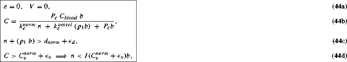
where

$$\begin{aligned} I(X)\;=\;\dfrac{P_{c}\;C_{blood}\;-\;X\;k^{vessel}_{c}\;p_{1}\;-\;X\;P_{c}}{X\;k^{norm}_{c}}. \end{aligned}$$

(45)

This state represents a tissue with normal cells, blood vessels and oxygen. The sum of normal cell density and vessel density exceeds the carrying capacity for normal cells thus blocking normal cell proliferation. Also the vessel density is such that it supplies enough oxygen ($C>C_{v}^{norm}+\epsilon _{v}>C_{a}^{norm}+\epsilon _{a}$), so that there is no normal cell death and no VEGF production leading to angiogenesis.

Case 3 :

In this case, $S_{tot}\!\,=n\!\,+\!\,(p_{1}\;b)\!\,>d_{tip}+\epsilon _{d}$. Since $d_{tip}+\epsilon _{d}\!\,>d_{norm}+\epsilon _{d}$, Eq. (33c) reduces to

$$\begin{aligned} \mathscr {H}(C_{a}^{norm}-C,\;\epsilon _{a})\;\beta _{norm}\;n\!\,=\!\,0, \end{aligned}$$

which holds either if $n\!\,=\!\,0 \text { or } C\!\,>C_{a}^{norm}+\epsilon _{a}$.

Case 3.1 :

Let $n\!\,=\!\,0$. Equation (33b) reduces to $\delta _{v}V\!\,=\!\,0$ implying $V\!\,=\!\,0$. These conditions lead to the steady state configuration given in Case 2.1 with an added condition, $S_{tot} = p_{1}b > d_{tip}+\epsilon _{d}$. However, $V=0$ satisfies Eq. (33d) irrespective of the value of $S_{tot}$. Hence, the extra condition is irrelevant.

Case 3.2 :

Let $C\!\,>C_{a}^{norm}+\epsilon _{a}$. From Eq. (43), we get

$$\begin{aligned} C\!\,=\!\,\dfrac{P_{c}\;C_{blood}\;b}{k^{norm}_{c}\;n\;+\;k^{vessel}_{c}\;(p_{1}\;b)\;+\;P_{c}\;b}. \end{aligned}$$

Rearranging the inequality $C>C_{a}^{norm}+\epsilon _{a}$, we can obtain a relation between n and b, as follows,

$$\begin{aligned} n < I(C_{a}^{norm}+\epsilon _{a}) b, \end{aligned}$$

(46)

where $I(C_{a}^{norm}+\epsilon _{a})$ is defined in Eq. (45). Also, from Eq. (33b), we obtain

$$\begin{aligned} V\!\,=\!\,\dfrac{\mathscr {H}(C_{v}^{norm}-C,\epsilon _{v})\;k_{v}^{norm}\;n}{P_{v}\;b\;+\;\delta _{v}}. \end{aligned}$$

(47)

Case 3.2.1 :

Thus, if $C\!\,>C_{v}^{norm}+\epsilon _{v}$, the steady state configuration becomes

$$\begin{aligned}&e\!\,=\!\,0,\quad V\!\,=\!\,0, \end{aligned}$$

(48a)

$$\begin{aligned}&C\!\,=\!\,\dfrac{P_{c}\;C_{blood}\;b}{k^{norm}_{c}\;n\;+\;k^{vessel}_{c}\;(p_{1}\;b)\;+\;P_{c}\;b}, \end{aligned}$$

(48b)

$$\begin{aligned}&n\!\,+\!\,(p_{1}\;b)\!\,>d_{tip}+\epsilon _{d}, \end{aligned}$$

(48c)

$$\begin{aligned}&C\!\,>C_{v}^{norm}+\epsilon _{v}\implies n\!\,<\!\,I(C_{v}^{norm}+\epsilon _{v})\;b, \end{aligned}$$

(48d)

where I(X) is defined in Eq. (45).

However, it is worth noting that when $e=0 \text { and } C>C_{v}^{norm}+\epsilon _{v}$, Eq. (33d) holds irrespective of $S_{tot}=n+(p_{1}b)>d_{tip}+\epsilon _{d}$. Hence, the condition given in Eq. (48c) is irrelevant. However, on omitting this condition, Eq. (33c) holds either if $n=0$, which leads to Case 2.1, or if $S_{tot}=n+(p_{1}b)>d_{norm}+\epsilon _{d}$, which leads to Case 2.2.2. Thus, the configuration obtained in Eq. (48) is not a new configuration.

Case 3.2.2 :

Next, when $C\!\,<C_{v}^{norm}+\epsilon _{v}$, we get

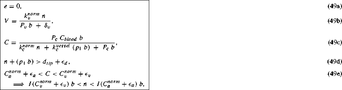
where I(X) is defined in Eq. (45).

This steady state represents a tissue with normal cells, blood vessels, oxygen and VEGF but no tip cells. The oxygen attains a certain concentration dictated by the blood vessel density and the normal cell density. This value of the concentration being below the threshold $C_{v}^{norm}+\epsilon _{v}$, causes hypoxic normal cells to secrete VEGF. However, the normal cells and the blood vessels occupy the entire space in the tissue thus preventing any further sprouting from the blood vessels in response to the VEGF signals. Similar to the oxygen concentration, the VEGF concentration reaches a certain steady concentration depending on the normal cell density and the blood vessel density.

References

Alarcón T, Byrne H, Maini P (2003) A cellular automaton model for tumour growth in inhomogeneous environment. J Theor Biol 225(2):257–274
Alarcón T, Byrne HM, Maini PK (2004) A mathematical model of the effects of hypoxia on the cell-cycle of normal and cancer cells. J Theor Biol 229(3):395–411
Alarcón T, Byrne HM, Maini PK (2005) A multiple scale model for tumor growth. Multiscale Model Simul 3(2):440–475
Alarcón T, Owen MR, Byrne HM, Maini PK (2006) Multiscale modelling of tumour growth and therapy: the influence of vessel normalisation on chemotherapy. Comput Math Methods Med 7(2–3):85–119
Anderson A, Rejniak K, Gerlee P, Quaranta V (2007) Modelling of cancer growth, evolution and invasion: bridging scales and models. Math Model Nat Phenom 2(3):1–29
Aubert M, Chaplain MAJ, McDougall SR, Devlin A, Mitchell CA (2011) A continuum mathematical model of the developing murine retinal vasculature. Bull Math Biol 73(10):2430–2451
Balding D, McElwain DLS (1985) A mathematical model of tumour-induced capillary growth. J Theor Biol 114(1):53–73
Betteridge R, Owen MR, Byrne HM, Alarcón T, Maini PK (2006) The impact of cell crowding and active cell movement on vascular tumour growth. Netw Heterog Media 1(4):515–535
Byrne HM, Chaplain MAJ (1995) Mathematical models for tumour angiogenesis: numerical simulations and nonlinear wave solutions. Bull Math Biol 57(3):461–486
Byrne HM, Chaplain MAJ (1998) Necrosis and apoptosis: distinct cell loss mechanisms in a mathematical model of avascular tumour growth. Comput Math Methods Med 1(3):223–235
Chaplain MAJ, Stuart AM (1991) A mathematical model for the diffusion of tumour angiogenesis factor into the surrounding host tissue. Math Med Biol 8(3):191–220
Connor AJ, Nowak RP, Lorenzon E, Thomas M, Herting F, Hoert S, Quaiser T, Shochat E, Pitt-Francis J, Cooper J et al (2015) An integrated approach to quantitative modelling in angiogenesis research. J R Soc Interface 12(110):20150–20546
Edelstein-Keshet L, Ermentrout B (1989) Models for branching networks in two dimensions. SIAM J Appl Math 49(4):1136–1157
Fisher RA (1937) The wave of advance of advantageous genes. Ann Eugen 7(4):355–369
Gaffney EA, Pugh K, Maini PK, Arnold F (2002) Investigating a simple model of cutaneous wound healing angiogenesis. J Math Biol 45(4):337–374
Gatenby RA, Gawlinski E (2001) Mathematical models of tumour invasion mediated by transformation-induced alteration of microenvironmental ph. In: Novartis foundation symposium, vol 1999. Wiley, Chichester, New York, pp 85–95
Larson DA (1978) Transient bounds and time-asymptotic behavior of solutions to nonlinear equations of fisher type. SIAM J Appl Math 34(1):93–104
McKean HP (1975) Application of brownian motion to the equation of Kolmogorov–Petrovskii–Piskunov. Commun Pure Appl Math 28(3):323–331
Mollison D (1977) Spatial contact models for ecological and epidemic spread. J R Stat Soc Ser B (Methodol) 39(3):283–326
Owen MR, Alarcón T, Maini PK, Byrne HM (2009) Angiogenesis and vascular remodelling in normal and cancerous tissues. J Math Biol 58:689–721
Owen MR, Stamper IJ, Muthana M, Richardson GW, Dobson J, Lewis CE, Byrne HM (2011) Mathematical modeling predicts synergistic antitumor effects of combining a macrophage-based, hypoxia-targeted gene therapy with chemotherapy. Cancer Res 71:2826–2837
Painter KJ, Hillen T (2002) Volume-filling and quorum-sensing in models for chemosensitive movement. Can Appl Math Q 10(4):501–543
Perfahl H, Byrne HM, Chen T, Estrella V, Alarcón T, Lapin A, Gatenby RA, Gillies RJ, Lloyd MC, Maini PK, Reuss M, Owen MR (2011) Multiscale modelling of vascular tumour growth in 3d: the roles of domain size and boundary conditions. PLoS ONE 6(4):e14,790
Ribba B, Colin T, Schnell S (2006) A multiscale mathematical model of cancer, and its use in analyzing irradiation therapies. Theor Biol Med Model 3(1):1
Royds J, Dower S, Qwarnstrom E, Lewis C (1998) Response of tumour cells to hypoxia: role of p53 and nfkb. Mol Pathol 51(2):55
Schnepf A, Roose T, Schweiger P (2008) Impact of growth and uptake patterns of arbuscular mycorrhizal fungi on plant phosphorus uptake—a modelling study. Plant Soil 312(1):85–99
Spill F, Guerrero P, Alarcon T, Maini PK, Byrne HM (2015) Mesoscopic and continuum modelling of angiogenesis. J Math Biol 70(3):485–532
Stokes AN (1976) On two types of moving front in quasilinear diffusion. Math Biosci 31(3):307–315
Stolarska MA, Kim Y, Othmer HG (2009) Multi-scale models of cell and tissue dynamics. Philos Trans R Soc Lond A Math Phys Eng Sci 367(1902):3525–3553
Author information
Authors and Affiliations
Corresponding author