
Abstract
This paper explores a single-parameter generalization of the Gini inequality measure. Taking the starting point to be the Borda-type social welfare function, which is known to generate the standard Gini measure, in which incomes (in ascending order) are weighted by their inverse rank, the generalisation uses a class of non-linear functions. These are based on the so-called ‘metallic sequences’ of number theory, of which the Fibonacci sequence is the best-known. The value judgements implicit in the measures are explored in detail. Comparisons with other well-known Gini measures, along with the Atkinson measure, are made. These are examined within the context of the famous ‘leaky bucket’ thought experiment, which concerns the maximum leak that a judge is prepared to tolerate, when making an income transfer from a richer to a poorer person. Inequality aversion is thus viewed in terms of being an increasing function of the leakage that is regarded as acceptable.


Data Availability
Not applicable Code availability. Not applicable
Notes
Indeed, a clear dichotomy can no longer be drawn between descriptive/statistical measures and so-called ‘ethical’ measures, since it is usually possible to identify implicit value judgements associated with earlier inequality measures; see, for example, Shorrocks (1988).
Other typical features of the type of social welfare function advanced by Atkinson include the properties of symmetry (welfare outcomes are independent of the precise personal identities of individuals), continuity (welfare does not change abruptly for small changes in individual welfare levels), and population-neutrality (the welfare function is invariant with respect to population replications).
Atkinson’s independently conceived notion of an ‘equally distributed equivalent’ income was in fact anticipated by Serge-Christophe Kolm (1969) in terms of what he called the ‘equivalent equal’ income.
Constant absolute aversion can be introduced by instead writing \({\Phi } \left (x_{i}\right ) =1-\exp \left (\beta x_{i}\right ) \), where β is constant absolute aversion, \(-{\Phi }^{\prime \prime }\left (x_{i}\right ) /{\Phi }^{\prime }\left (x_{i}\right ) \). In addition, an intermediate case is given by \({\Phi } \left (x_{i}\right ) =\left (x_{i}+x_{0}\right )^{1-\varepsilon }/\left (1-\varepsilon \right ) \) for ε≠ 1. However, these alternatives have received little attention compared with the constant relative inequality aversion case used by Atkinson.
Their result was based on a result by Stuart (1954) on the correlation between values and ranks in samples from continuous distributions.
Muliere and Scarsini (1989) showed that if the contribution of any v-tuple of individuals is equal to the income of the poorest person, the average social welfare of all v-tuples is \(\bar {x}\left (1-G\left (v\right ) \right ) \), namely the abbreviated function discussed below. For practical computations, it is not advisable to use the covariance form for v > 2, as the resulting \(G\left (v\right ) \) may not be monotonic: see Schechtman and Zitikis (2006, p. 390). On calculations, see also Schechtman and Yitzhaki (2008).
The French mathematician Jean-Charles de Borda (1733–1799) proposed, in 1781, in the context of a voting system where candidates are ranked by voters, a points scoring system in which options are given scores equal to their reverse rank positions. Aggregation of scores over all voters then gives the winner as the one with the highest total score. The properties of the ‘Borda Rule’, and its application to a variety of aggregation settings (including committee decisions, social welfare judgements, and normative indicators such as poverty, inequality, real national income) have been intensively investigated by Sen (1977).
For example, Kakwani (1980) used the form, \(\widetilde {W}=\bar {x}/\left (1+G\right ) \), while Dagum (1990) used \(\widetilde {W}=\bar {x}\left (1-G\right ) /\left (1+G\right ) \). These are examined in detail in Creedy and Hurn (1999). Shorrocks (1988) used \(\widetilde {W}=\bar {x}\exp (I),\) while de V. Graaff (1977) suggested \(\widetilde {W}=\bar {x}\left (1-I\right )^{\theta }\).
Although it was known much earlier, the series \(f_{1}\left (i\right ) \) is named after the Italian mathematician Leonardo Bonacci (1170–approx 1240), better known simply as Fibonacci. The series \(f_{2}\left (i\right ) \) is named after the English mathematician, John Pell (1611–1685), although again it was known before Pell. It is also sometimes known as the Pell-Lucas series, after the French mathematician Francois Lucas (1842–1891).
Furthermore, these are special cases of the Generalised secondary Fibonacci sequence given by: a,b,pb + qa,p(pb + qa) + qb, and so on, for which \(f\left (i\right ) /f\left (i-1\right ) \) approaches \(0.5\left (p+\sqrt {p^{2}+4q} \right ) \).
The relationship between \(A\left (\varepsilon \right ) \) and ε is examined in detail in Creedy (2019).
Figure 3 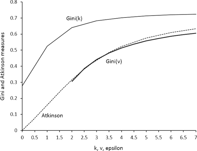
Alternative Gini and Atkinson Measures for Hypothetical Distribution
However, there are slight differences in this small-population case.
Table 2 Leak Tolerated, in cents, When Transfering One Dollar to Lower-Ranked Person: Extended Gini For a very useful text on the mathematics of metallic sequences, see Koshy (2001).

References
Amiel, Y., Creedy, J. and Hurn, S. (1999). Measuring attitudes towards inequality. Scandinavian J. Econ. 101, 83–96.
Atkinson, A.B. (1970). On the measurement of inequality. J. Public Econ. 2, 244–263.
Borda, J.C. (1781). Memoires sur les elections au scrutin. Memoires des l’Academie Royale des Sciences. English translation by A. de Graza. Isis. 44.
Chakravarty, S.R. (1988). Extended Gini indices of inequality. Int. Econ. Rev. 29, 147–56.
Chameni Nembua, C. (2006). Linking Gini to entropy: measuring Inequality by an interpersonal class of indices. Econ. Bullet. 4, 1–9.
Chameni Nembua, C. (2008). Measuring and explaining economic inequality: An extension of the Gini coefficient. MPRA Paper No. 31242. Available online at https://mpra.ub.uni-muenchen.de/31242/.
Creedy, J. (2019). The Atkinson inequality measure and inequality aversion. Victoria University of Wellington Chair of Public Finance Working Paper, WP01/209.
Creedy, J. and Hurn, S. (1999). Distributional preferences and the extended Gini Measure of inequality. In Advances in Econometrics, Income Distribution and Scientific Methodology:Essays in Honor of Camilo Dagum, (D.J. Slottje, eds.). Physica, New York.
Dagum, C. (1990). On the relationship between income inequality measures and social welfare functions. J. Econ. 43, 91–102.
de V. Graaff, J. (1977). Equity and efficiency as components of the general welfare. South African J. Econ. 45, 362–375.
Donaldson, D. and Weymark, J.A. (1980). A single parameter generalization of the Gini indices of inequality. J. Econ. Theory 22, 67–86.
Kakwani, N.C. (1980). On a class of poverty measures. Econometrica48, 437–446.
Kolm, S.C. (1969). The Optimum Production of Social Justice. In Public Economics, (J. Margolis and H. Guitton, eds.). Macmillan, London.
Koshy, T. (2001). Fibonacci and Lucas Numbers with Applications. Wiley, New York.
Lasso de la Vega, C. and Seidl, C. (2007). The impossibility of a just Pigouvian. ECINEQ WP 2007–69.
Lerman, R.I. and Yitzhaki, S. (1984). A note on the calculation and interpretation of the Gini index. Econ. Lett. 15, 363–368.
Muliere, P. and Scarsini, M. (1989). A note on stochastic dominance and inequality measures. J. Econ. Theory 49, 314–323.
Sen, A.K. (1973). On Economic Inequality. Oxford University Press, Oxford.
Sen, A.K. (1977). Social choice theory: a re-examination. Econometrica45, 53–89.
Schechtman, E. and Yitzhaki, S. (2008). Calculating the extended Gini coefficient from grouped data: a covariance presentation. Bullet. Stat. Econ. 2, 64–69.
Schechtman, E. and Zitikis, R. (2006). Gini indices as areas and covariances: what is the difference between the two representations? METRON – International Journal of Statistics. LXIV 385–397.
Shorrocks, A.F. (1988). Aggregation Issues in Inequality Measurement. In Measurement in Economics: Theory and Application of Economic Indices, (W. Eichhorn ed.). Physica, Hiedelberg.
Shorrocks, A.F. and Slottje, D. (2002). Approximating unanimity orderings: an application to Lorenz dominance. Journal of Economics Zeitschrift fur Nationalokonomie, Supplement 9, 91–117.
Stuart, A. (1954). The correlation between variate-values and ranks in samples from a continuous distribution. British J. Stat. Psychol. 7, 37–44.
Subramanian, S. (2021). A single-parameter generalization of Gini based on the ‘metallic’ sequence of number theory. Econ. Bull. 41, 2309–2319.
Tibiletti, L. and Subramanian, S. (2015). Inequality aversion and the extended Gini in the light of a two-person cake-sharing problem. J. Human Develop. Capabilit. 16, 237–244.
Yitzhaki, S. (1983). On an extension of the Gini inequality index. Int. Econ. Rev. 24, 617–628.
Acknowledgments
We are grateful to the referees for helpful suggestions.
Funding
Creedy’s work on this paper is part of a project on ‘Measuring Income Inequality, Poverty, and Mobility in New Zealand’, funded by an Endeavour Research Grant from the Ministry of Business, Innovation and Employment (MBIE) and awarded to the Chair in Public Finance at Victoria University of Wellington. Subramanian did not receive support from any organization for the submitted work.
Author information
Authors and Affiliations
Corresponding author
Ethics declarations
Conflict of Interest
The authors have no conflicts of interest to declare that are relevant to the content of this article.
Additional information
Publisher’s Note
Springer Nature remains neutral with regard to jurisdictional claims in published maps and institutional affiliations.
We are grateful to the referees for helpful suggestions.
Appendix: Derivation of the Pell Index of Inequality
Appendix: Derivation of the Pell Index of Inequality
This appendix provides a short derivation of the metallic ratio expression for the ‘Pell Index’ of inequality, denoted G2 above and shown in equation (3.10). The derivation makes use of the following two standard results relating to the Pell number sequence: Footnote 15
- (a):
-
The n th term of the Pell sequence, \(P\left (n\right ) \), can be approximated by \(\delta ^{n}/\left (2\sqrt {2}\right ) \), where δ is the ‘silver ratio’, \(\delta =1+\sqrt {2}\).
- (b):
-
The sum of the first n Pell numbers, \({\sum }_{i=1}^{n}P\left (i\right ) \), is \([ 3P\left (n\right ) +P\left (n-1\right ) -1] /2\). In terms of the approximation in (a) and after some manipulation, this can be written as:
$$ {\sum}_{i=1}^{n}P\left( i\right) =\frac{\delta^{n-1}\left( 3\delta +1\right) -2\sqrt{2}}{4\sqrt{2}} $$(A.1)
Using (16), the Pell inequality index is derived from the function, W2. Write WP = W2, and using the notation introduced in Section 3, for any ordered n-vector of incomes \(\mathbf {x=}\left (x_{1},...,x_{n}\right ) \):
Making use of result (b) stated above, this becomes:
The equally distributed equivalent, xE,P, using (17), is given by:
Using, again, result (b) stated above:
But \({\sum }_{i=1}^{n}\delta ^{n-i}=\left (\delta ^{n}-1\right ) /\sqrt {2}\), and making the appropriate substitution yields:
Using (A.3), (A.4) and (A.6), the equally distributed equivalent is:
This simplifies to:
The Pell index is the proportional deviation of the equally distributed equivalent income from the arithmetic mean, \(G_{P}=1-x_{E,P}/\bar {x}\). Using (A.8), this gives the result in equation (3.10).
As a check, the exact value of the Fibonacci and Pell inequality indices, as given in equation (3.16), can be compared with the ‘metallic ratio’ approximations as given by equations (3.9) and (3.10) respectively, for a hypothetical income distribution. Consider the ten-person ordered distribution \(\left (20,30,50,55,60,75,90,120,140\right ) \) used in Section 3.3 above. It turns out that, for this distribution, the exact and approximate values, as given by (3.6), for k = 1, and (3.9) respectively for the Fibonacci index are 0.5325 and 0.5255. The corresponding exact and approximate values for the Pell index, given by (3.6), for k = 2, and (3.10) respectively, are 0.6404 and 0.6441.
Rights and permissions
Springer Nature or its licensor (e.g. a society or other partner) holds exclusive rights to this article under a publishing agreement with the author(s) or other rightsholder(s); author self-archiving of the accepted manuscript version of this article is solely governed by the terms of such publishing agreement and applicable law.
About this article

Cite this article
Creedy, J., Subramanian, S. Exploring A New Class of Inequality Measures and Associated Value Judgements: Gini and Fibonacci-Type Sequences. Sankhya B 85, 110–131 (2023). https://doi.org/10.1007/s13571-023-00302-y
Received:
Accepted:
Published:
Issue Date:
DOI: https://doi.org/10.1007/s13571-023-00302-y
Keywords
- Income inequality
- Gini coefficient, extensions of Gini
- social welfare functions
- equally distributed equivalent income
- Atkinson
- inequality aversion
- value judgements
- efficiency and equity
- leaky bucket experiment.