
Abstract
Texture features play a vital role in land cover classification of remotely sensed images. Local binary pattern (LBP) is a texture model that has been widely used in many applications. Many variants of LBP have also been proposed. Most of these texture models use only two or three discrete output levels for pattern characterization. In the case of remotely sensed images, texture models should be capable of capturing and discriminating even minute pattern differences. So a multivariate texture model is proposed with four discrete output levels for effective classification of land covers. Remotely sensed images have fuzzy land covers and boundaries. Support vector machine is highly suitable for classification of remotely sensed images due to its inherent fuzziness. It can be used for accurate classification of pixels falling on the fuzzy boundary of separation of classes. In this work, texture features are extracted using the proposed multivariate descriptor, MDLTP/MVAR that uses multivariate discrete local texture pattern (MDLTP) supplemented with multivariate variance (MVAR). The classification accuracy of the classified image obtained is found to be 93.46 %.
1 Introduction
Land cover refers to the biophysical attributes of the surface of the earth. Features of land covers include texture, shape, colour, contrast and so on. Land cover classification involves classifying the multispectral remotely sensed image into various land covers such as land, vegetation, water, etc. Some of the applications of land cover classification are town planning, conservation of earth’s natural resources, studying the effects of climatic conditions and analyzing change in land forms. Identification of a suitable feature extraction technique and classifier is a challenging task in land cover classification of remotely sensed images.
Texture based methods are widely used in applications like face recognition, content based image retrieval, pattern classification in medical imagery and land cover classification of remotely sensed images. Texture is a surface property that characterizes the coarseness and smoothness of land covers. Pixel based techniques classify a pixel depending on the intensity of the current pixel but texture based techniques classify a pixel based on its relationship with the neighborhood. Texture measures can capture micro as well as macro patterns as they can be captured by varying the size of neighborhood. Most of the texture based methods are rotation, illumination, scaling and color invariant and are robust and susceptible to noise. Recent texture based studies reveal that texture measures augmented with a contrast measure characterizing the local neighborhood yield accurate results, provided the conditions like using a sufficient number of precise samples for training, a suitable neighborhood for finding pattern unit and an optimal window size are satisfied.
Support vector machine (SVM) is basically a binary classifier but can be used for multiclass classification following suitable approaches. The advantage of SVM over other classifiers is that SVM allows a marginal region on both sides of the linear or non linear boundary of separation of classes and classifies the pixels within the support regions based on measures of uncertainty and reliability. This ensures that uncertain pixels that fall in the support or boundary region are assigned exactly correct class labels. The objective of this research work is to propose a multivariate texture model that performs land cover classification of remotely sensed images with the help of SVM.
1.1 Motivation and justification of the proposed approach
A variety of texture models are found in literatures. The univariate texture model, local binary pattern (LBP) [11] was proposed for gray level images and its classification accuracy was proved to be better in many applications. A multivariate extension of the univariate LBP model was proposed for remotely sensed images by [10] as multivariate local binary pattern (MLBP). They concluded that MLBP model with uncertainty measure helped in identifying objects and yielded high classification accuracy. Algorithms using wavelet transform [2] and rotation invariant features of Gabor wavelets [3] were proposed for performing texture segmentation of gray level images and they reported that the results were promising. To provide better pattern discrimination, advanced local binary pattern (ALBP) [1] was proposed for texture classification and applied on standard texture databases. It was proved that ALBP characterized local and global texture information and was robust in discriminating texture. Local texture pattern (LTP) [15] was proposed for gray level images and later extended to remotely sensed images as multivariate local texture pattern (MLTP) [16]. From the experiments, it was proved that MLTP model gave high classification accuracy. In dominant local binary pattern (DLBP) [8] histograms of dominant patterns were used as features for texture classification of standard textures. Local derivative pattern [13] was proposed for face recognition under challenging image conditions. A novel face descriptor named local color vector binary pattern (LCVBP) [7] was proposed to recognize face images with challenges. Two color local texture features like color local Gabor wavelets (CLGWs) and color local binary pattern (CLBP) [4] were purposed for face recognition and both were combined to maximize their complementary effect of color and texture information respectively.
Among many classification algorithms used for texture based classification of remotely sensed images, support vector machine [[6], [12]], relevance vector machine [5] are reported often in literatures. [6] suggested that SVM was more suitable for heterogeneous samples for which only a few number of training samples were available. [12] concluded that the SVM classification approach was better than K nearest neighbour classification algorithm. [9] performed a detailed survey of various classification algorithms including pixel based, sub pixel based, parametric, non parametric, hard and soft classification algorithms. They summarized that the success of an image classification algorithm depended on the availability of high quality remotely sensed imagery, the design of a proper classification procedure and analyst’s skills.
Among the texture models mentioned earlier, only LBP, LTP, wavelet and Gabor wavelet have been extended to remotely sensed images already. The challenge in spectral methods is that they produce features of high dimensionality. So dimensionality reduction may be required prior to classification. At the same time, the multivariate texture models MLBP [10] and MLTP [17] yield high classification accuracy on remotely sensed images using at most three discrete levels. So it is expected that if we increase the number of discrete levels, we can more precisely model the relationship between neighbour pixels. Motivated by this, a multivariate texture model with four discrete levels is proposed for land cover classification of remotely sensed images. Incorporating fuzziness either during feature extraction [18] and [14] or classification can improve the classification accuracy of pattern classification and recognition problems. Support vector machine is a fuzzy classifier often used in classification of remotely sensed images. Moreover it converges quickly and needs only a minimum number of samples for classification. Justified by these facts, the proposed multivariate texture model is combined with SVM classification algorithm for performing land cover classification of remotely sensed images. The objective of this research work is to propose a multivariate texture model MDLTP for land cover classification of remotely sensed images that gives high classification accuracy.
1.2 Outline of the proposed approach
The proposed approach has texture feature extraction part as shown in Fig. 1a and classification part as shown in Fig. 1b. During feature extraction, the centre pixel of each 3 × 3 neighbourhood of a sample is assigned a pattern label using the proposed local texture descriptor. Local contrast variance is also used as a supplementary local feature descriptor. These two local descriptors are then used to form a 2D global histogram of each sample. The 2D global histograms thus formed characterize the global feature of the sample. The SVM classifier works in two phases as shown in Fig. 1b. In the training phase, training samples are extracted from distinct land cover classes of remotely sensed images. Texture features in the form of 2D global histograms of training samples are used to train SVM classifier. In the testing phase, test samples centred around each pixel of remotely sensed image are extracted, 2D global histogram was found and given as input to SVM. The SVM classifier finds the optimal hyper plane of separation and returns the class label based on its prior learning of training samples.

Feature extraction and classification
1.3 Organization of the paper
The second section of the paper gives the overview of the proposed multivariate texture model. The third section describes the SVM classification algorithm. The fourth section gives a detailed account of the experiments conducted with the proposed multivariate texture model for supervised texture classification of remotely sensed image. It also evaluates the performance of the proposed model. The final section discusses the outcomes of various experiments and gives the conclusion.
2 Texture feature extraction
2.1 Local texture description using discrete local texture pattern (DLTP)
The proposed texture model extracts local texture information from a neighbourhood in an image. Let us take a 3 × 3 neighbourhood where g c , g 1, ···g 8 be the pixel values of a local region where the value of the centre pixel is g c and g 1, g 2···g 8 are the pixel values in its neighbourhood. The relationship between the centre pixel and one of its neighbour pixels is described in Eq. (1).
Here ‘m’ is the threshold which is set to express the closeness of neighbouring pixel with the centre pixel. The value p(g i , g c )stands for output level assigned to ith pixel in the neighbourhood. The discrete output levels are fixed numerically to −1, 0, 1 and 9 to assign unique pattern values during individual summation of positive and negative values. The output levels characterize the neighbourhood pixel relation. Concatenation of these levels in a neighbourhood gives us a pattern unit. The sample calculation of pattern unit for m = 5 is shown below.
The total number of patterns considering all combinations of four output levels with number of pixels in the neighbourhood (P) equal to eight will be 48. This will lead to increase in number of bins required when these local patterns are accumulated to characterize global regions. In order to reduce the number of possible patterns, a uniformity measure (U) is introduced as defined in Eq. (3). It corresponds to the number of circular spatial transitions between output levels like −1, 0, 1 and 9 in the pattern unit. Patterns for which U value is less than or equal to three are considered uniform and other patterns are considered non uniform. The gray scale DLTP for local region ‘X’ is derived as in Eq. (2). The value PS stands for sum of all positive output levels including zero and NS stands for sum of all negative output levels in the pattern unit. To each pair of (NS+1, PS+1) values, a unique DLTP value is obtained from the lookup table ‘L’ for all uniform patterns and 166 will be assigned for non uniform patterns.
where
where s(x,y) = \( \left\{ \begin{gathered} 1\quad if\quad \left| {x\; - \;y} \right|\; > \;0 \hfill \\ 0\quad if\quad otherwise \hfill \\ \end{gathered} \right. \)and
The lookup table (L) shown in Table 1 provides unique pattern values to the different combinations of NS+1 and PS+1 values. The maximum negative sum (NS) is eight as there can be eight −1’s. The maximum positive sum (PS) is 72 as there can be eight 9’s. So the size of the lookup table is (9 × 73). All entries in the table are filled sequentially starting from 1 to 165 which characterize unique pattern labels. Zero entries in the lookup table show that the patterns will never occur. This scheme provides 165 uniform patterns and one non uniform pattern.
2.2 Local contrast variance- supplementary feature
Texture features by itself do not capture contrast information of an image. This will result in patterns with same texture values but different contrast values to get classified into same class. In order to avoid this, texture is supplemented with contrast information. Rotation invariant local variance is a powerful spatial property that provides contrast information and is defined for 3 × 3 neighbourhood of a gray scale image as follows.
Equal percentile binning is performed for quantization of variance values. We can find the bin interval for binning variance values by using the formula `100/B’, where B is the required number of bins.
2.3 Extending DLTP and VAR for multispectral bands
The proposed DLTP operator for gray scale image is extended as Multivariate DLTP (MDLTP). Among the multispectral bands, three most suitable bands for land cover classification are chosen and combined to form a RGB image. Nine DLTP operators are calculated in the RGB image. Out of nine, three DLTP operators (RR, GG and BB) describe the local texture in each of the three bands R, G and B individually. Six more DLTP operators describe the local texture of the cross relation of each band with other bands (GR, BR, RG, BG, RB and GB). For example, the GR cross relation is obtained by replacing the centre pixel of R band in its neighbourhood with the centre pixel of G band. Nine DLTP operators thus obtained are arranged in a 3 × 3 matrix. Then MDLTP is found by calculating DLTP for the 3 × 3 resulting matrix as shown below. This MDLTP histogram has only 166 bins.
where ‘i’ ranges from 0 to 7 (total number of pixels in 3 × 3 neighbourhood).
The univariate variance measure (VAR) can be extended as Multivariate variance (MVAR) for remotely sensed image as follows. The individual independent variances VAR1, VAR2 and VAR3 of R, G and B bands are found using Eq. (5) and combined into a single composite variance (MVAR) by applying the formula below.
2.4 Global description through 2D histogram
The multivariate local descriptor describes the texture pattern over any local region. The global description of an image can be obtained through combining multivariate local texture descriptor and multivariate local contrast variance in a 2D histogram. The steps are given below.
-
1.
Find multivariate local texture descriptor (MDLTP) and multivariate local contrast variance descriptor (MVAR) for all pixels by using a sliding window neighbourhood that runs over the image from top left to bottom right.
-
2.
Compute the occurrence frequency of the ordered pair MDLTP and MVAR into a 2D histogram where x ordinate denotes MDLTP and y ordinate denotes MVAR.
3 Support vector machine classification algorithm
The SVM classifier is a supervised binary classifier which can classify pixels that are not linearly separable. Support vectors are the samples closest to the separating hyper plane and SVM orientates this hyper plane in such a way as to be as far as possible from the sure candidates of both classes. The optimization problem of finding support vectors with maximal margin around separating hyper plane is solved subject to a tolerance value entered by the user. The classifier solves optimization problem with the help of one of the kernels like linear, sigmoid, radial basis function, polynomial, wavelet and frame. Each new testing sample is classified by evaluating the sign of output of SVM.
Multiclass classification is done in SVM following two approaches namely one against one and one against all. We have used one against one approach in this article. In one against one approach, one SVM per each pair of classes is used. The whole set of patterns is divided into two classes at a time and finally the patterns which get classified into more than one class are fixed to a single class using probability measures. The steps involved in multiclass classification are as follows.
3.1 Training phase
-
1.
If ‘n’ is the number of classes (In Fig. 2, Cl1, Cl2 …. Cln are classes), then ‘nC2’ support vector machines are needed.
Fig. 2 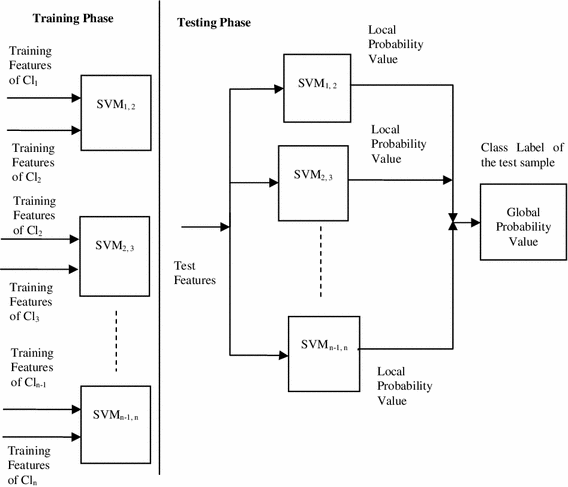
Working principle of SVM
-
2.
Each SVM is trained with the 2D histograms of known samples and their class labels (pertaining to the corresponding pair of classes).

3.2 Testing phase
-
1.
The 2D global histogram of unknown sample is given as input to all SVM’s.
-
2.
The output of SVM per pair of classes is mapped to a local probability value.
-
3.
Then the global posterior probability is found from the individual probabilities to decode the class label of the unknown sample.
The overall working principle of multiclass SVM is outlined in Fig. 2.
4 Experiments and results
4.1 Experimental data
The remotely sensed image under study is a IRS P6, LISS- IV image supplied by National Remote Sensing Centre(NRSC), Hyderabad, Government of India. The image has been taken in July 2007 and is of size 2959x2959. It is formed by combining bands 2, 3 and 4 of LISS- IV data (Green, red and near IR) and is shown in Fig. 3. It covers the area in and around Tirunelveli city located in the state of Tamil Nadu in India. It extends to the suburbs of Nanguneri village in the South, the outskirts of Palayamkottai in the East, the suburbs of Alankulam village in the North and the suburbs of Cheranmahadevi village near Ambasamudram in the West. The river Thamirabarani runs across the diagonal region of the image. In the image, residential areas are either with closely packed buildings or with partially occupied buildings with shrubs and trees scattered then and there. Some irrigation tanks are present inside the city. Also in the south of Tirunelveli city leading to Nanguneri village several irrigation tanks and vegetation areas are present. In the North, bare soil is scattered in some places on the way to Sankarankoil. In the West, on the way leading to Cheranmahadevi fertile paddy fields and vegetation are present on either sides of the perennial river. An updated geological map has been selected as a reference for ground truth study of the same area.

IRS P6, LISS-IV remotely sensed image
The experimental classes or training samples are the areas of interest extracted from source image in Fig. 3 and are of size 16 × 16 as shown below Table 2.
4.2 Land cover classification of remotely sensed image with MDLTP/MVAR
In experiments, the size of training and testing samples are kept same to get high classification accuracy. Since the size of the training sample was 16 × 16, the size of testing sample was also fixed to 16 × 16. The multivariate local texture feature (MDLTP) and multivariate local contrast variance (MVAR) were found and the 2D histograms for global description were formed for all samples as illustrated in Sect. 2. In training phase, the 2D histograms of training samples were used to train SVM. In testing phase, the 2D histograms of testing samples were given as input to SVM. The classifier returned the class label. The classified image is shown in Fig. 4.

Classified image using MDLTP/MVAR
The MDLTP/MVAR model discriminates well between various land covers because it is so designed to assign distinct and precise pattern codes to capture patterns. So settlement and vegetation-3 classes cluster densely. The thin diagonal line of water running across the image is clearly traced without discontinuity. The vegetation-1 class which lies on either sides of river is seen vividly. The vegetation-2 class present around water tanks is classified precisely.
4.3 Performance evaluation of classified image
The overall classification accuracy and Kappa coefficient are the performance metrics for assessing the classified image. To compute these values, an error matrix is built as follows. The size of error matrix is ‘c × c’ where ‘c’ is the number of classes. If a pixel that belongs to class (where 1≤ i ≤c) is correctly classified, then a count is added in entry (i, i) of error matrix. If a pixel that belongs to class ci is incorrectly classified to class (where 1≤ j ≤c), then a count is added to the entry (i, j) of error matrix. The diagonal entries mark correct classifications while the upper and lower diagonal entries mark incorrect classifications. Then the overall accuracy (Po) can be found as follows.
where ‘b’ is the total number of observations and
xii is the observation in row ‘i’ and column ‘i’ of error matrix.
The classification accuracy expected (Pe) is found as below.
where x1 is the marginal total of row ‘i’ and x2 is the marginal total of column ‘i’. Kappa coefficient is found using Po and Pe as follows.
In our experiments, a set of stratified random samples comprising of 2400 pixels were used for building error matrix. The performance measures Po and kappa coefficient described above are found for the classified image in Fig. 4 and shown in Table 3 and Table 4 respectively.
The proposed model MDLTP/MVAR gives a classification accuracy of 93.46 % and a kappa coefficient of 0.9156. The model performs well because the neighbourhood pixel relations are precisely captured with the help of four discrete levels.
For evaluating the performance of the proposed model with the existing pixel based and texture based classification algorithms, the classification accuracies of various algorithms were found and tabulated in Table 5. The existing texture methods such as gabor wavelet, multivariate local binary pattern (MLBP), multivariate local texture pattern (MLTP) and wavelet and the existing pixel based methods such as Maximum likelihood classifier, Mahalonobis distance classifier and minimum distance classifier are considered for comparison.(Table 5)
From the above table, it is inferred that the pixel based classifiers give classification accuracy only in the order of 75 %. This is due to the lack of attaching due weightage to the intensities of neighbourhood rather than just the intensity of current pixel value. The performance of spectral models drops when the spectral characteristics of different patterns are similar. The MLBP texture model gives 90.42 % classification accuracy. The degree of quantization is more in MLBP as we use only two discrete levels for modeling neighbour pixel relation. Moreover, MLTP (with discrete levels like 0, 1 and 9) with MVAR yield 91.88 % classification accuracy. The proposed model MDLTP/MVAR performs better than the chosen methods and gives 93.46 % classification accuracy.
5 Discussion and conclusion
A multivariate texture model (MDLTP) is proposed for land cover classification of remotely sensed images. The advantages of the proposed model are threefold. Firstly, it gives stable results even for small window sizes and secondly, it requires only a minimum number of training samples in training phase. Thirdly, it captures additional uniform patterns. The model is made wholesome by adding contrast variance as supplementary measure. The significance of the method is vividly seen as it captures even minute pattern differences with the help of four discrete levels and subsequent assignment of unique pattern labels. The SVM classifier augments the texture model by incorporating fuzziness in classifying land covers. From the experiments, it is proved that the proposed model yields 93.46 % classification accuracy.
In future, it is proposed to extend the model for hyper spectral data. The proposed model will certainly inspire researchers to find optimal number of discrete levels for each texture model so that maximum classification accuracy can be achieved. The model can be hybridized with extreme learning machine or relevance vector machine classifier to yield better classification accuracy.
References
Liao, Chung CS (2007) Texture classification by using advanced local binary patterns and spatial distribution of dominant patterns. Acoust Speech Signal Process IEEE Int Conf ICASSP 2007. doi:10.1109/ICASSP.2007.366134
Arivazhagan S, Ganesan L (2003) Texture segmentation using wavelet transform. Pattern Recogn Lett 24(16):3197–3203
Arivazhagan S, Ganesan L, Priyal S (2006) Texture classification using Gabor wavelets based rotation invariant features. Pattern Recogn Lett 27(16):1976–1982
Choi JY, Ro YM, Plataniotis KN (2012) Color local texture features for color face recognition. IEEE Trans Image Process 21(3):1366–1380
Demir, Ertuirk (2007) Hyperspectral image classification using Relevence Vector Machines. IEEE Geosci Remote Sens Lett 4(4):586–590
Hermes, Frieauff, Puzicha (1999) Support Vector Machines for Land Usage Classification in Landsat TM imagery. Proc IEEE Geosci Remote Sens Soc 1:348–350
Lee SH, Choi JY, Ro YM, Plataniotis KN (2012) Local color vector binary patterns from multichannel face images for face recognition. IEEE Trans Image Process 21(4):2347–2353
Liao S, Law WK, Chung CS (2009) Dominant local binary patterns for texture classification. IEEE Trans Image Process 18(5):1107–1118
Lu D, Weng Q (2007) A survey of image classification methods and techniques for improving classification performance. Int J Remote Sens 28(5, 10):823–870
Lucieer, Stein, Fisher (2005) Multivariate texture-based segmentation of remotely sensed imagery for extraction of objects and their uncertainty. Int J Remote Sens 26(14):2917–2936
Ojala, Pietikainen, Maenpaa (2001) A generalized local binary pattern operator for multiresolution gray scale and rotation invariant texture classification. advances in. Pattern Recogn 2013:399–408
Ge QZ, Ling, Qiong (2008). High efficient classification on SVM. International archives of the photogrammetry, remote sensing and spatial information sciences. Vol. XXXVII. Part B2, Beijing
Raju USN, Sridhar Kumar A, Mahesh B, Reddy E (2010) Texture classification with high order local pattern descriptor: local derivative pattern. Glob J Comput Sci Technol 10(8):72–76
Srinivasan EM, Ramar K, Suruliandi A (2011) Texture analysis using local texture patterns: a fuzzy logic approach. Int J Pattern Recognit Artif Intell 25(5):741–762
Surliandi A, Ramar K (2008) Local texture patterns- a univariate texture model for classification of images. ADCOM 2008:14–17. doi:10.1109/ADCOM.2008.4760424
Suruliandi A (2009). A study on classification of remotely sensed multispectral mages-a textural approach. Ph.D dissertation work submitted to Manonmaniam Sundaranar University, Tamil Nadu, India
Suruliandi A, Jenicka S (2014). Texture based classification of remotely sensed images. In: Int J (ed) Signal Imaging Syst Eng. Inderscience, (today in press, Accepted for publication in Sep 2013, Abstract available online in Forthcoming Articles)
Dimitris K, Iakovidis, Eystratios G, Keramidas, and Dimitris Maroulis (2008). Fuzzy local binary patterns for ultrasound texture characterization. ICIAR 2008. Lecture notes in computer science. vol 5112. Springer, Heidelberg, pp 750–759
Author information
Authors and Affiliations
Corresponding author
Rights and permissions
About this article

Cite this article
Jenicka, S., Suruliandi, A. A textural approach for land cover classification of remotely sensed image. CSIT 2, 1–9 (2014). https://doi.org/10.1007/s40012-014-0038-4
Received:
Accepted:
Published:
Issue Date:
DOI: https://doi.org/10.1007/s40012-014-0038-4