Data Collection and Preliminary Data Analysis

Abstract

This chapter starts by presenting some basic notions and characteristics of different types of data collection systems and types of sensors. Next, simple ways of validating and assessing the accuracy of the data collected are addressed. Subsequently, salient statistical measures to describe univariate and multivariate data are presented along with how to use them during basic exploratory data and graphical analyses. The two types of measurement uncertainty (bias and random) are discussed and the concept of confidence intervals is introduced and its usefulness illustrated. Finally, three different ways of determining uncertainty in a data reduction equation by propagating individual variable uncertainty are presented; namely, the analytical, numerical and Monte Carlo methods.

Problems

Pr. 3.1

Consider the data given in Table. 3.2. Determine

• (a) the 10% trimmed mean value

• (b) which observations can be considered to be “mild” outliers (> 1.5 × IQR)

• (c) which observations can be considered to be “extreme” outliers (> 3.0 × IQR)

• (d) identify outliers using Chauvenet’s criterion given by Eq. 3.19

• (e) compare the results from (b), (c) and (d).

Pr. 3.2

Consider the data given in Table. 3.6. Perform an exploratory data analysis involving computing pertinent statistical summary measures, and generating pertinent graphical plots.

Pr. 3.3

A nuclear power facility produces a vast amount of heat which is usually discharged into the aquatic system. This heat raises the temperature of the aquatic system resulting in a greater concentration of chlorophyll which in turn extends the growing season. To study this effect, water samples were collected monthly at three stations for one year. Station A is located closest to the hot water discharge, and Station C the farthest (Table 3.13).

Table 3.13 Data table for Problem 3.3

You are asked to perform the following tasks and annotate with pertinent comments:

• (a) flag any outlier points

• (b) compute pertinent statistical descriptive measures

• (c) generate pertinent graphical plots

• (d) compute the correlation coefficients.

Pr. 3.4

Consider Example 3.7.3 where the uncertainty analysis on chiller COP was done at full load conditions. What about part-load conditions, especially since there is no collected data? One could use data from chiller manufacturer catalogs for a similar type of chiller, or one could assume that part-load operation will affect the inlet minus the outlet chilled water temperatures (∆T) in a proportional manner, as stated below.

• (a) Compute the 95% CL uncertainty in the COP at 70% and 40% full load assuming the evaporator water flow rate to be constant. At part load, the evaporator temperatures difference is reduced proportionately to the chiller load, while the electric power drawn is assumed to increase from a full load value of 0.8 kW/t to 1.0 kW/t at 70% full load and to 1.2 kW/t at 40% full load.

• (b) Would the instrumentation be adequate or would it be prudent to consider better instrumentation if the fractional COP uncertainty at 95% CL should be less than 10%.

• (c) Note that fixed (bias) errors have been omitted from the analysis, and some of the assumptions in predicting part-load chiller performance can be questioned. A similar exercise with slight variations in some of the assumptions, called a sensitivity study, would be prudent at this stage. How would you conduct such an investigation?

Pr. 3.5

Consider the uncertainty in the heat transfer coefficient illustrated in Example 3.7.1. The example was solved analytically using the Taylor’s series approach. You are asked to solve the same example using the Monte Carlo method:

• (a) using 500 data points

• (b) using 1000 data points

Compare the results from this approach with those in the solved example.

Pr. 3.6

You will repeat Example 3.7.6. Instead of computing the standard deviation, plot the distribution of the time variable t in order to evaluate its shape. Numerically determine the uncertainty bands for the 95% CL.

Pr. 3.7

Determining cooling coil degradation based on effectiveness

The thermal performance of a cooling coil can also be characterized by the concept of effectiveness widely used for thermal modeling of traditional heat exchangers. In such coils, a stream of humid air flows across a coil supplied by chilled water and is cooled and dehumidified as a result. In this case, the effectiveness can be determined as:

$$ \varepsilon= \frac{{{\rm{actual\; heat\; transfer \;rate}}}}{{{\rm{maximum \;possible\; heat\; transfer\; rate}}}}{\rm{ = }}\frac{{({h_{ai}} - {h_{ao}})}}{{({h_{ai}} - {h_{ci}})}} $$

(3.41)

where h _ai and h _ao are the enthalpies of the air stream at the inlet and outlet respectively, and h _ci is the enthalpy of entering chilled water.

The effectiveness is independent of the operating conditions provided the mass flow rates of air and chilled water remain constant. An HVAC engineer would like to determine whether the coil has degraded after it has been in service for a few years. For this purpose he assembles the following coil performance data at identical air and water flow rates corresponding to when originally installed (done during start-up commissioning) and currently (Table 3.14).

Table 3.14 Data table for Problem 3.7

Note that the uncertainty in determining the air enthalpies are relatively large due to the uncertainty associated with measuring bulk air stream temperatures and humidities. However, the uncertainty in the enthalpy of the chilled water is only half of that of air.

• (a) Asses, at 95% CL, whether the cooling coil has degraded or not. Clearly state any assumptions you make during the evaluation.

• (b) What are the relative contributions of the uncertainties in the three enthalpy quantities to the uncertainty in the effectiveness value? Do these differ from the installed period to the time when current tests were performed?

Pr. 3.8

Consider a basic indirect heat exchanger where heat rates of the heat exchange associated with the cold and hot sides is given by:

$$ {Q_{actual}} = {m_c}.{c_{pc}}.({T_{c,o}} - {T_{c,i}})\quad({\rm{cold}}\;{\rm{side}}\;{\rm{heating}}) $$

(3.42a)

$${Q_{actual}} = {m_h}.{c_{ph}}.({T_{h,i}}-{T_{h,o}})\quad({\rm{hot}}\;{\rm{side}}\;{\rm{cooling}})$$

where m, T and c are the mass flow rate, temperature and specific heat respectively, while the subscripts 0 and i stand for outlet and inlet, and c and h denote cold and hot streams respectively.

The effectiveness of the sensible heat exchanger is given by:

$$ \begin{aligned}\varepsilon&= \frac{{{\rm{actual\; heat\; transfer\; rate}}}}{{{\rm{maximum\; possible\; heat\; transfer\; rate}}}}\\&=\frac{{{Q_{actual}}}}{{{{(m{c_p})}_{\min }}({T_{hi}} - {T_{ci}})}} \end{aligned}$$

(3.42b)

Assuming the values and uncertainties of various parameters shown in the table (Table 3.15):

Table 3.15 Parameters and uncertainties to be assumed (Pr. 3.8)

• (i) compute the heat exchanger loads and the uncertainty ranges for the hot and cold sides

• (ii) compute uncertainty in the effectiveness determination

• (iii) what would you conclude regarding the heat balance checks?

Pr. 3.9

The following table (Table 3.16) (EIA 1999) indicates the total electricity generated by five different types of primary energy sources as well as the total emissions associated by each. Clearly coal and oil generate a lot of emissions or pollutants which are harmful not only to the environment but also to public health. France, on the other hand, has a mix of 21% coal and 79% nuclear.

Table 3.16 Data table for Problem 3.9

• (a) Calculate the total and percentage reductions in the three pollutants should the U.S. change its power generation mix to mimic that of France (Hint: First normalize the emissions per kWh for all three pollutants)

• (b) The generation mix percentages (coal, oil, natural gas, nuclear and hydro/wind) have an inherent uncertainty of 5% at the 95% CL, while the uncertainties of the three pollutants are 5, 8 and 3% respectively. Assuming normal distributions for all quantities, compute the uncertainty of the reduction values estimated in (a) above.

Pr. 3.10

Uncertainty in savings from energy conservation retrofits

There is great interest in implementing retrofit measures meant to conserve energy in individual devices as well as in buildings. These measures have to justified economically, and including uncertainty in the estimated energy savings is an important element of the analysis. Consider the rather simple problem involving replacing an existing electric motor with a more energy efficient one. The annual energy savings E_save in kWh/yr are given by:

$$ {E_{save}} = (0.746).({\textit{HP}}).(Hours).\left( {\frac{1}{{{\eta _{old}}}} - \frac{1}{{{\eta _{new}}}}} \right) $$

(3.43)

with the symbols described in Table 3.17 along with their numerical values.

Table 3.17 Data table for Problem 3.10

• (i) Determine the absolute and relative uncertainties in E_save under these conditions.

• (ii) If this uncertainty had to be reduced, which variable will you target for further refinement?

• (iii) What is the minimum value of ${\eta _{new}}$ under which the lower bound of the 95% CL interval is greater than zero.

Pr. 3.11

Uncertainty in estimating outdoor air fraction in HVAC systems

Ducts in heating, ventilating and air-conditioning (HVAC) systems supply conditioned air (SA) to the various spaces in a building, and also exhaust the air from these spaces, called return air (RA). A sketch of an all-air HVAC system is shown in Fig. 3.39. Occupant comfort requires that a certain amount of outdoor air (OA) be brought into the HVAC systems while an equal amount of return air is exhausted to the outdoors. The OA and the RA mix at a point just before the air-handler unit. Outdoor air ducts have dampers installed in order to control the OA since excess OA leads to unnecessary energy wastage. One of the causes for recent complaints from occupants has been identified as inadequate OA, and sensors installed inside the ducts could modulate the dampers accordingly. Flow measurement is always problematic on a continuous basis. Hence, OA flow is inferred from measurements of the air temperature T_R inside the RA stream, of T_O inside the OA stream and T_M inside the mixed air (MA) stream. The supply air is deduced by measuring the fan speed with a tachometer, using a differential pressure gauge to measure static pressure rise, and using manufacturer equation for the fan curve. The random error of the sensors is 0.2°F at 95% CL with negligible bias error.

Fig. 3.39

Sketch of an all-air HVAC system supplying conditioned air to indoor rooms of a building

• (a) From a sensible heat balance where changes in specific heat with temperature are neglected, derive the following expression for the fraction of outdoor air fraction (ratio of outdoor air and mixed air) ${\rm{O}}{{\rm{A}}_{\rm{f}}} = ({T_R} - {T_M})/({T_R} - {T_O})$

• (b) Derive the expression for the uncertainty in OA_f and calculate the 95% CL in the OA_f if T_R = 70°F, T_O = 90°F and T_M = 75°F.

Pr. 3.12

Sensor placement in HVAC ducts with consideration of flow non-uniformity

Consider the same situation as in Pr. 3.11. Usually, the air ducts have large cross-sections. The problem with inferring outdoor air flow using temperature measurements is the large thermal non-uniformity usually present in these ducts due to both stream separation and turbulence effects. Moreover, temperature (and, hence density) differences between the OA and MA streams result in poor mixing. The following table gives the results of a traverse in the mixed air duct with 9 measurements (using an equally spaced grid of 3 × 3 designated by numbers in bold in Table 3.18). The measurements were replicated four times under the same outdoor conditions. The random error of the sensors is 0.2°F at 95% CL with negligible bias error. Determine:

Table 3.18 Table showing the temperature readings (in °F) at the nine different sections (S#1–S#9) of the mixed air (MA) duct (Pr. 3.12)

• (a) the worst and best grid locations for placing a single sensor (to be determined based on analyzing the recordings at each of the 9 grid locations and for all four time periods)

• (b) the maximum and minimum errors at 95% CL one could expect in the average temperature across the duct cross-section, if the best grid location for the single sensor was adopted.

Pr. 3.13

Uncertainty in estimated proportion of exposed subjects using Monte Carlo method

Dose-response modeling is the process of characterizing the relation between the dose of an administered/exposed agent and the incidence of an adverse health effect. These relationships are subject to large uncertainty because of the paucity of data as well as the fact that they are extrapolated from laboratory animal tests. Haas (2002) suggested the use of an exponential model for mortality rate due to inhalation exposure by humans to anthrax spores (characterized by the number of colony forming units or cfu):

$$ p = 1 - \exp ( - kd) $$

(3.44)

where p is the expected proportion of exposed individuals likely to die, d is the average dose (in cfu) and k is the dose response parameter (in units of 1/cfu). A value of k = 0.26 × 10⁻⁵ has been suggested. One would like to determine the shape and magnitude of the uncertainty distribution of d at p = 0.5 assuming that the one standard deviation (or uncertainty) of k is 30% of the above value and is normally distributed. Use the Monte Carlo method with 1000 trials to solve this problem. Also, investigate the shape of the error probability distribution, and ascertain the upper and lower 95% CL.

Pr. 3.14

Uncertainty in the estimation of biological dose over time for an individual

Consider an occupant inside a building in which an accidental biological agent has been released. The dose (D) is the cumulative amount of the agent to which the human body is subjected, while the response is the measurable physiological change produced by the agent. The widely accepted approach for quantifying dose is to assume functional forms based on first-order kinetics. For biological and radiological agents where the process of harm being done is cumulative, one can use Haber’s law (Heinsohn and Cimbala 2003):

$$ D(t) = k\int\limits_{{t_1}}^{{t_2}} {C(t)dt}$$

(3.45a)

where C(t) is the indoor concentration at a given time t, k is a constant which includes effects such as the occupant breathing rate, the absorption efficiency of the agent or species,… and t₁ and t₂ are the start and end times. This relationship is often used to determine health-related exposure guidelines for toxic substances. For a simple one-zone building, the free response, i.e., the temporal decay is given in terms of the initial concentration C(t₁) by:

$$ C(t) = C({t_1}).\exp [( - a(t - {t_1})] $$

(3.45b)

where the model parameter “a” is a function of the volume of the space and the outdoor and supply air flow rates. The above equation is easy to integrate during any time period from t₁ to t₂, thus providing a convenient means of computing total occupant inhaled dose when occupants enter or leave the contaminated zones at arbitrary times. Let a = 0.017186 with 11.7% uncertainty while C(t₁) = 7000 cfu/m³ (cfu–colony forming units). Assume k = 1.

• (a) Determine the total dose to which the individual is exposed to at the end of 15 min.

• (b) Compute the uncertainty of the total dose at 1 min time intervals over 15 min (similar to the approach in Example 3.7.6)

• (c) Plot the 95% CL over 15 min at 1 min intervals

Pr. 3.15

Propagation of optical and tracking errors in solar concentrators

Solar concentrators are optical devices meant to increase the incident solar radiation flux density (power per unit area) on a receiver. Separating the solar collection component (viz., the reflector) and the receiver can allow heat losses per collection area to be reduced. This would result in higher fluid operating temperatures at the receiver. However, there are several sources of errors which lead to optical losses:

• (i) Due to non-specular or diffuse reflection from the reflector, which could be due to improper curvature of the reflector surface during manufacture (shown in Fig. 3.40a) or to progressive dust accumulation over the surface over time as the system operates in the field;

  Fig. 3.40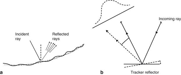

  

  Different types of optical and tracking errors. a Micro-roughness in solar concentrator surface leads to a spread in the reflected radiation. The roughness is illustrated as a dotted line for the ideal reflector surface and as a solid line for the actual surface. b Tracking errors lead to a spread in incoming solar radiation shown as a normal distribution. Note that a tracker error of ${\sigma _{track}}$ results in a reflection error ${\sigma _{\textit {reflec}}} = 2.{\sigma _{track}}$ from Snell’s law. Factor of 2 also pertains to other sources based on the error occurring as light both enters and leaves the optical device (see Eq. 3.46)

• (ii) Due to tracking errors arising from improper tracking mechanisms as a result of improper alignment sensors or non-uniformity in drive mechanisms (usually, the tracking is not continuous; a sensor activates a motor every few minutes which re-aligns the reflector to the solar radiation as it moves in the sky). The result is a spread in the reflected radiation as illustrated in Fig. 3.40b;

• (iii) Improper reflector and receiver alignment during the initial mounting of the structure or due to small ground/pedestal settling over time).

The above errors are characterized by root mean square (or rms) random errors (bias errors such as that arising from structural mismatch can often be corrected by one-time or regular corrections), and their combined effect can be determined statistically following the basic propagation of errors formula. Note that these errors need not be normally distributed, but such an assumption is often made in practice. Thus, rms values representing the standard deviations of these errors are used for such types of analysis.

The finite angular size of the solar disc results in incident solar rays that are not parallel but subtend an angle of about 33 min or 9.6 mrad.

• (a) You will analyze the absolute and relative effects of this source of radiation spread at the receiver considering various other optical errors described above, and using the numerical values shown in Table 3.19.

  $$\begin{aligned}{\sigma _{totalspread}} & = [{({\sigma _{solardisk}})^2} + {(2{\sigma _{manuf}})^2} + {(2{\sigma _{dustbuild}})^2} \\ & \quad+ {[{(2{\sigma _{sensor}})^2} + {(2{\sigma _{drive}})^2} + {({\sigma _{rec - misalign}})^2}]^{1/2}}\end{aligned}$$

  (3.46)

• (b) Plot the variation of the total error as a function of the tracker drive non-uniformity error for three discrete values of dust building up (0, 1 and 2 mrad).

Table 3.19 Data table for Problem 3.15

References

Abbas, M., and J.S. Haberl,1994. “Development of indices for browsing large building energy databases”, Proc. Ninth Symp. Improving Building Systems in Hot and Humid Climates, pp. 166–181, Dallas, TX, May.
ANSI/ASME,1990. “Measurement Uncertainty: Instruments and Apparatus”, ANSI/ASME Standard PTC 19.1–1985, American Society of Mechanical Engineers, New York, NY.
ASHRAE 14, 2002. Guideline 14–2002: Measurement of Energy and Demand Savings, American Society of Heating, Refrigerating and Air-Conditioning Engineers, Atlanta.
ASHRAE, 2005. Guideline 2–2005: Engineering Analysis of Experimental Data, American Society of Heating, Refrigerating and Air-Conditioning Engineers, Atlanta, GA.
Ayyub, B.M. and R.H. McCuen,,1996. Numerical Methods for Engineers, Prentice-Hall, Upper Saddle River, NJ
Belsley, D.A., E. Kuh and R.E. Welsch 1980, Regression Diagnostics, John Wiley & Sons, New York
Braun, J.E., S.A. Klein, J.W. Mitchell and W.A. Beckman,1989. Methodologies for optimal control of chilled water systems without storage, ASHRAE Trans., 95(1), American Society of Heating, Refrigerating and Air-Conditioning Engineers, Atlanta, GA.
Cleveland, W.S.,1985. The Elements of Graphing Data, Wadsworth and Brooks/Cole, Pacific Grove, California.
Coleman, H.W. and H.G. Steele,1999. Experimentation and Uncertainty Analysis for Engineers, 2nd Edition, John Wiley and Sons, New York.
Dorgan, C.E. and J.S. Elleson,1994. Design Guide for Cool Thermal Storage, American Society of Heating, Refrigerating and Air-Conditioning Engineers, Atlanta, GA.
Devore J., and N. Farnum, 2005. Applied Statistics for Engineers and Scientists, 2nd Ed., Thomson Brooks/Cole, Australia.
Doebelin, E.O.,1995. Measurement Systems: Application and Design, 4th Edition, McGraw-Hill, New York
EIA, 1999. Electric Power Annual 1999, Vol.II, October 2000, DOE/EIA-0348(99)/2, Energy Information Administration, US DOE, Washington, D.C. 20585–065 http://www.eia.doe.gov/eneaf/electricity/epav2/epav2.pdf.
Glaser, D. and S. Ubbelohde, 2001. “Visualization for time dependent building simulation”, 7th IBPSA Conference, pp. 423–429, Rio de Janeiro, Brazil, Aug. 13–15.
Haas, C. N., 2002. “On the risk of mortality to primates exposed to anthrax spores.” Risk Analysis vol. 22(2): pp.189–93.
Haberl, J.S. and M. Abbas, 1998. Development of graphical indices for viewing building energy data: Part I and Part II, ASME J. Solar Energy Engg., vol. 120, pp. 156–167
Heinsohn, R.J. and J.M. Cimbala, 2003, Indoor Air Quality Engineering, Marcel Dekker, New York, NY
Holman, J.P. and W.J. Gajda, 1984. Experimental Methods for Engineers, 5th Ed., McGraw-Hill, New York
Kreider, J.K., P.S. Curtiss and A. Rabl, 2009. Heating and Cooling of Buildings, 2nd Ed., CRC Press, Boca Raton, FL.
Reddy, T.A., 1990. Statistical analyses of electricity use during the hottest and coolest days of summer for groups of residences with and without air-conditioning. Energy, vol. 15(1): pp. 45–61.
Schenck, H., 1969. Theories of Engineering Experimentation, 2nd Edition, McGraw-Hill, New York.
Tufte, E.R.,1990. Envisioning Information, Graphic Press, Cheshire, CN.
Tufte, E.R., 2001. The Visual Display of Quantitative Information, 2nd Edition, Graphic Press, Cheshire, CN
Tukey, J., 1988. The Collected Works of John W. Tukey, W. Cleveland (Editor), Wadsworth and Brookes/Cole Advanced Books and Software, Pacific Grove, CA
Wonnacutt, R.J. and T.H. Wonnacutt,1985. Introductory Statistics, 4th Ed., John Wiley & Sons, New York.
Author information
Authors and Affiliations
Corresponding author