
Abstract
Trapdoor functions (TDFs) are a fundamental primitive in cryptography. Yet, the current set of assumptions known to imply TDFs is surprisingly limited, when compared to public-key encryption. We present a new general approach for constructing TDFs. Specifically, we give a generic construction of TDFs from any Chameleon Encryption (Döttling and Garg [CRYPTO’17]) satisfying a novel property which we call recyclability. By showing how to adapt current Computational Diffie-Hellman (CDH) based constructions of chameleon encryption to yield recyclability, we obtain the first construction of TDFs with security proved under the CDH assumption. While TDFs from the Decisional Diffie-Hellman (DDH) assumption were previously known, the possibility of basing them on CDH had remained open for more than 30 years.
Research supported in part from DARPA/ARL SAFEWARE Award W911NF15C0210, AFOSR Award FA9550-15-1-0274, AFOSR YIP Award, DARPA and SPAWAR under contract N66001-15-C-4065, a Hellman Award and research grants by the Okawa Foundation, Visa Inc., and Center for Long-Term Cybersecurity (CLTC, UC Berkeley). The views expressed are those of the author and do not reflect the official policy or position of the funding agencies.
You have full access to this open access chapter, Download conference paper PDF
Keywords
1 Introduction
Trapdoor functions (TDFs) are a fundamental primitive in cryptography, historically pre-dating the complexity-based development of public key encryption (PKE) [11, 28]. Informally, TDFs are a family of functions, where each function in the family is easy to compute given the function’s index key, and also easy to invert given an associated trapdoor key. The security requirement is that a randomly chosen function from the family should be hard to invert without knowledge of a trapdoor key.
A salient difference between TDFs and PKE lies in their inversion (decryption) algorithms: while the inversion algorithm of a TDF recovers the entire pre-image in full, the decryption algorithm of a PKE only recovers the corresponding plaintext, and not necessarily the randomness. This full-input recovery feature of TDFs is useful in may applications. For example, suppose we have two image points \(y_1:= \mathsf {F} (\mathsf {ik} _1, x_1)\) and \(y_2:= \mathsf {F} (\mathsf {ik} _2, x_2)\) of a trapdoor function \(\mathsf {F} \), and we want to convince \(\mathsf {Alice}\) — who is given both \(y_1\) and \(y_2\) but only a trapdoor key \(\mathsf {tk} _1\) for \(\mathsf {ik} _1\) — that \(x_1 = x_2\). This will be easy for \(\mathsf {Alice}\) to do herself: retrieve \(x_1\) from \(y_1\) using the trapdoor key \(\mathsf {tk} _1\) and check whether \(y_1 = \mathsf {F} (\mathsf {ik} _1, x_1)\) and \(y_2 = \mathsf {F} (\mathsf {ik} _2, x_1)\).Footnote 1 This is a very useful property, especially in the context of chosen-ciphertext (CCA2) security, and is in fact the main reason behind the success of building CCA2-secure PKE in a black-box way from various forms of TDFs [23, 27, 29]. In contrast, enabling this technique based on PKE [25] requires the use of expensive non-interactive zero knowledge proofs [4, 16], which in turn require strong assumptions and lead to non-black-box constructions.
The deterministic structure of TDFs, however, comes with a price, making the construction of TDFs more challenging than that of PKE. This belief is justified by an impossibility result of Gertner, Malkin and Reingold [18] showing that TDFs cannot be built from PKE in a black-box way. As another evidence, while it was known from the 80’s how to build semantically-secure PKE from the Decisional Diffie-Hellman (DDH) assumption [15, 20, 32], it took two decades to realize TDFs based on DDH [27].
Despite the fundamental nature of TDFs and extensive research on this notion [1,2,3, 17, 23, 27, 29, 31] a long-standing question has remained open:

The main difficulty of the above question is that all known DDH-based constructions of TDFs, e.g., [17, 27], exploit properties of DDH, such as pseudorandomness of low rank matrices of group elements, which do not hold in the CDH setting (see Sect. 1.1).
Apart from being a natural question, it has the following theoretical motivation: since we know that TDFs are not necessary in a black-box sense for PKE [18], there may be computational assumptions that imply PKE but not TDFs. Thus, it is important to understand whether TDFs can be obtained from all existing computational assumptions that imply PKE. This provides insights into the hardness nature of TDFs as well as our computational assumptions.
1.1 Lack of CDH-Based Techniques for TDF
Diffie-Hellman related assumptions (even DDH) do not naturally lend themselves to a TDF construction. The main reason why it is more difficult to build TDFs from such assumptions, compared to, say, factoring related assumptions, is that we do not know of any generic trapdoors for the discrete log problem. Indeed, a long standing open problem in cryptography is whether PKE can be based on the sole hardness of the discrete log problem. To see how this makes things more difficult, consider ElGamal encryption: to encrypt a group element \(g_m\) under a public key \((g, g_1)\), we return \((g^r, g_1^r \cdot g_m)\), where r is a random exponent. The decryption algorithm can recover \(g_m\) but not r because computing r is as hard as solving the discrete log problem.
Known DDH-based TDF constructions [17, 27] get around the above obstacle by designing their TDFs in such a way that during inversion, one will only need to solve the discrete log problem over a small space, e.g., recovering a bit b from \(g^b\). The main idea is as follows: the index key \(\mathsf {ik} \) of their TDF is \(g^{\mathsf {M}}\), where g is a generator of the group \(\mathbb {G}\) of order p and \(\mathsf {M} \in {\mathbb Z}_p^{n \times n}\) is a random \(n \times n\) invertible matrix and \(g^{\mathsf {M}}\) denotes entry-wise exponentiation. Let \(\mathsf {tk}:= \mathsf {M}^{-1}\) be the trapdoor key. Using \(\mathsf {ik} \), the evaluation algorithm on input \(\mathsf {x} \in \{0,1\}^n\) may use the algebraic property of the group to compute \(\mathsf {y}:= g^{\mathsf {M} \mathsf {x}} \in \mathbb {G}^n\). Now using \(\mathsf {tk} \) and \(\mathsf {y}\) one can compute \(g^\mathsf {x} \in \mathbb {G}^n\), hence retrieving \(\mathsf {x}\).
To argue about one-wayness, one uses the following property implied by DDH: the matrix \(g^{\mathsf {M}}\) is computationally indistinguishable from a matrix \(g^{\mathsf {M}_1}\), where \(\mathsf {M}_1\) is a random matrix of rank one. If the index key is now set to \(g^{\mathsf {M}_1}\) and if we have \(2^n \gg p\), then even an unbounded adversary cannot retrieve the original \(\mathsf {x}\) from \(\mathsf {y}\). This argument is used to establish one-wayness for the TDF.
Unfortunately, the above rank indistinguishability property used to prove one-wayness is not known (and not believed) to be implied by CDH. Thus, designing TDFs based on CDH requires new techniques.
Finally, we mention that even from the Computational Bilinear Assumption [6] (i.e., pairing-based CDH) no TDF constructions are known. The closest is a result of Wee [30], showing that trapdoor relations, which are much weaker than TDFs, can be built from CDH. Roughly, trapdoor relations are a relaxed version of TDFs, in that the function might not be efficiently computable on individual points but one may sample efficiently a random input element together with its corresponding image.
1.2 Our Results and Techniques
We give the first construction of TDFs under the CDH assumption. Our construction is black-box and is obtained through a general construction of TDFs from a primitive we call a recyclable one-way function with encryption (OWFE). Moreover, we show that an adaptive strengthening of our notion of recyclable OWEF yields a black-box construction of CCA2-secure PKE.
An OWFE is described by a one-way function \(\mathsf {f}_{\mathsf {pp}} :\{0,1\}^n \rightarrow \{0,1\}^\nu \), where \(\mathsf {pp}\) is a public parameter, together with encapsulation/decapsulation algorithms \((\mathsf {E}, \mathsf {D})\). Specifically, \(\mathsf {E}\) takes as input \(\mathsf {pp}\), an image \(\mathsf {y}\in \{0,1\}^\nu \) of \(\mathsf {f}_{\mathsf {pp}}\), an index \(i \in [n]\) and a selector bit \(b \in \{0,1\}\), and produces an encapsulated ciphertext \(\mathsf {ct} \) and a corresponding key bit \(\mathsf {e} \in \{0,1\}\). The algorithm \(\mathsf {D}\) allows anyone to retrieve \(\mathsf {e}\) from \(\mathsf {ct} \) using any pre-image \(\mathsf {x}\) of \(\mathsf {y}\) whose ith bit is b. For security, letting \(\mathsf {y}:= \mathsf {f}_{\mathsf {pp}}(\mathsf {x})\), we require if \((\mathsf {ct}, \mathsf {e}) \xleftarrow {\$}\mathsf {E}(\mathsf {pp}, \mathsf {y}, (i,b)) \) and \(\mathsf {x}_i \ne b\), then even knowing \(\mathsf {x}\) one cannot recover \(\mathsf {e}\) from \(\mathsf {ct} \) with probability better than \(\textstyle {\frac{1}{2}}+ \mathsf{negl}(\lambda )\), where \(\lambda \) is the security parameter. That is, for any \(\mathsf {x}\in \{0,1\}^n\), \(i \in [n]\), we have \((\mathsf {x}, \mathsf {ct}, \mathsf {e}) {\mathop {\equiv }\limits ^{c}} (\mathsf {x}, \mathsf {ct}, \mathsf {e}')\), where \(\mathsf {e}' \xleftarrow {\$}\{0,1\}\), \((\mathsf {ct},\mathsf {e}) \xleftarrow {\$}\mathsf {E}(\mathsf {pp}, \mathsf {f}(\mathsf {pp}, \mathsf {x}), (i, 1-\mathsf {x}_i))\) and \({\mathop {\equiv }\limits ^{c}} \) denotes computational indistinguishability. Our OWFE notion is a weakening of the hash encryption notion [13] in that we do not require \(\mathsf {f}\) to be collision resistant. The following is a variant of the CDH-based construction of [13].
CDH-based instantiation of OWFE [13]. Let \(\mathbb {G}\) be a group of prime order p. The public parameter is a \(2 \times n\) matrix of random group elements  and \(\mathsf {y}:= \mathsf {f}(\mathsf {pp}, \mathsf {x}\in \{0,1\}^n) = \displaystyle \prod _{j \in [n]}^{} g_{j,\mathsf {x}_j}\).
To perform \(\mathsf {E}(\mathsf {pp}, \mathsf {y}, (i ,b))\), sample \(\rho \xleftarrow {\$}{\mathbb Z}_p \) and return \((\mathsf {ct}, \mathsf {e})\), where

and \(\mathsf {e}:= \mathsf {HC}(\mathsf {y}^\rho )\), where \(\mathsf {HC}\) is a hardcore bit function. The function \(\mathsf {D}\) is now derived easily. See the main body for the proof of security.
Recyclability. Our recyclability notion asserts that the ciphertext part output, \(\mathsf {ct} \), of the key encapsulation algorithm \(\mathsf {E}\) is independent of the corresponding image input part \(\mathsf {y}\). That is, letting \(\mathsf {E}_1\) and \(\mathsf {E}_2\) refer to the first and second output of \(\mathsf {E}\), for any values of \(\mathsf {y}_1\) and \(\mathsf {y}_2\), we always have \(\mathsf {E}_1(\mathsf {pp}, \mathsf {y}_1 ,(i, b);\rho ) = \mathsf {E}_1(\mathsf {pp}, \mathsf {y}_2 , (i, b);\rho )\). It is easy to verify that the above CDH-based OWFE satisfies this property. Thus, we may drop \(\mathsf {y}\) as an input to \(\mathsf {E}_1\) and obtain the following:
Property 1. Letting \(\mathsf {x}\in \{0,1\}^n\), \(\mathsf {x}_i = b\), \(\mathsf {ct}:= \mathsf {E}_1(\mathsf {pp}, (i,b); \rho )\) and \(\mathsf {y}:= \mathsf {f}(\mathsf {pp}, \mathsf {x})\):
1.3 Sketch of Our OWFE-Based Construction and Techniques
Let \((\mathsf {K}, \mathsf {f}, \mathsf {E}, \mathsf {D})\) be a recyclable OWFE scheme.Footnote 2 Our TDF construction is based on a new technique that we call bits planting. Briefly, the input \(\mathsf {X}\) to our TDF consists of a domain element \(\mathsf {x}\in \{0,1\}^n\) of \(\mathsf {f}(\mathsf {pp}, \cdot )\) and a blinding string  , for some r that we will specify later. The output \(\mathsf {Y}\) is comprised of \(\mathsf {y}:= \mathsf {f}(\mathsf {pp}, \mathsf {x})\), as well as a matrix of bits in which we copy all the bits of \({\mathbf {\mathsf{{b}}}}\) in the clear but in hidden spots determined by \(\mathsf {x}\); we fill up the rest of the matrix with key bits that somehow correspond to bit-by-bit encryption of \(\mathsf {x}\) under \(\mathsf {y}\). To an adversary, the matrix is “unrevealing,” with no indicative signs of what spots corresponding to the blinding part — which contain \({\mathbf {\mathsf{{b}}}}\) in the clear. However, using our designed trapdoor, an inverter can pull out both \(\mathsf {x}\) and \({\mathbf {\mathsf{{b}}}}\) from \(\mathsf {Y}\) with all but negligible probability.
Warm-up Construction. We first give a warm up construction in which our inversion algorithm only recovers half of the input bits (on average). Our TDF input is of the form \((\mathsf {x}, {\mathbf {\mathsf{{b}}}}) \in \{0,1\}^n \times \{0,1\}^n\). This warm-up construction contains most of the ideas behind the full-blown construction.
-
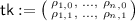
Key generation: The trapdoor key is
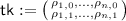 a matrix of randomness values, and the index key is
 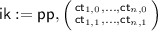 , formed as: $$\begin{aligned} \mathsf {ik}:=\mathsf {pp}, \begin{pmatrix} \mathsf {ct} _{1,0}:= \mathsf {E}_1(\mathsf {pp}, (1, 0); \rho _{1,0}), \ldots , \mathsf {ct} _{n,0}:= \mathsf {E}_1(\mathsf {pp}, (n,0);\rho _{n,0}) \\ \mathsf {ct} _{1,1}:= \mathsf {E}_1(\mathsf {pp}, (1, 1); \rho _{1,1}), \ldots , \mathsf {ct} _{n,1}:= \mathsf {E}_1(\mathsf {pp}, (n,1);\rho _{n,1}) \end{pmatrix}. \end{aligned}$$
 -
Evaluation \(\mathsf {F} (\mathsf {ik}, \mathsf {X})\): Parse
 and parse the input \(\mathsf {X} \) as \((\mathsf {x}\in \{0,1\}^n, {\mathbf {\mathsf{{b}}}}:= \mathsf {b}_1 \cdots \mathsf {b}_n \in \{0,1\}^n)\). Set \(\mathsf {y}:= \mathsf {f}(\mathsf {pp}, \mathsf {x})\). For \(i \in [n]\) set \(\mathsf {M}_i\) as follows: $$\begin{aligned} \mathsf {M}_i:= \begin{pmatrix} \mathsf {D}(\mathsf {pp}, \mathsf {x}, \mathsf {ct} _{i,0}) \\ \mathsf {b}_i \end{pmatrix} {\mathop {=}\limits ^{*}} \begin{pmatrix} \mathsf {E}_2(\mathsf {pp}, \mathsf {y}, (i, 0); \rho _{i,0}) \\ \mathsf {b}_i \end{pmatrix} \text {if~} \mathsf {x}_i = 0 \nonumber \\ \mathsf {M}_i:= \begin{pmatrix} \mathsf {b}_i \\ \mathsf {D}(\mathsf {pp}, \mathsf {x}, \mathsf {ct} _{i,1}) \end{pmatrix} {\mathop {=}\limits ^{*}} \begin{pmatrix} \mathsf {b}_i \\ \mathsf {E}_2(\mathsf {pp}, \mathsf {y}, (i, 1); \rho _{i,1}) \end{pmatrix}\text {if~} \mathsf {x}_i = 1 \end{aligned}$$(1)
The matrix \(\mathsf {M}_i\) is computed using the deterministic algorithm \(\mathsf {D}\) and the equalities specified as \({\mathop {=}\limits ^{*}}\) follow by Property (1).
Return \(\mathsf {Y}:= (\mathsf {y}, \mathsf {M}_1 || \dots || \mathsf {M}_n)\).
-
Inversion \(\mathsf {F^{-1}} (\mathsf {tk}, \mathsf {Y})\): Parse \(\mathsf {Y}:= (\mathsf {y}, \mathsf {M}_1 || \dots || \mathsf {M}_n)\) and
 . Set $$\begin{aligned} (\mathsf {M}' _1 || \dots ||\mathsf {M}'_n):= \begin{pmatrix} \mathsf {E}_2(\mathsf {pp}, \mathsf {y}, (1, 0); \rho _{1,0}), \ldots , \mathsf {E}_2(\mathsf {pp}, \mathsf {y}, (n, 0); \rho _{n,0}) \\ \mathsf {E}_2(\mathsf {pp}, \mathsf {y}, (1, 1); \rho _{1,1}), \ldots , \mathsf {E}_2(\mathsf {pp}, \mathsf {y}, (n, 1); \rho _{n,1}) \end{pmatrix}. \end{aligned}$$(2)
Output \((\mathsf {x}, {\mathbf {\mathsf{{b}}}}:= \mathsf {b}_1 \dots \mathsf {b}_n)\), where we retrieve \(\mathsf {x}_i\) and \(\mathsf {b}_i\) as follows. If \(\mathsf {M}'_{i,1} = \mathsf {M}_{i,1}\) and \(\mathsf {M}'_{i,2} \ne \mathsf {M}_{i,2}\) (where \(\mathsf {M}_{i, 1}\) is the first element of \(\mathsf {M}_i\)), then set \(\mathsf {x}_i:= 0\) and \(\mathsf {b}_i:= \mathsf {M}_{i,2} \). If \(\mathsf {M}'_{i,1} \ne \mathsf {M}_{i,1}\) and \(\mathsf {M}'_{i,2} = \mathsf {M}_{i,2}\), then set \(\mathsf {x}_i:= 1\) and \(\mathsf {b}_i:= \mathsf {M}_{i,1} \). Else, set \(\mathsf {x}_i:= \bot \) and \(\mathsf {b}_i:= \bot \).
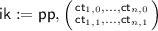
 a matrix of randomness values, and the index key is
  , formed as:
  and parse the input
  . Set
. Set One-Wayness (Sketch). We show \((\mathsf {ik}, \mathsf {Y}) {\mathop {\equiv }\limits ^{c}} (\mathsf {ik}, \mathsf {Y}_{\mathrm {sim}})\), where \((\mathsf {ik}, \mathsf {Y})\) is as above and
Noting that we may produce \((\mathsf {ik}, \mathsf {Y}_{\mathrm {sim}})\) using only \(\mathsf {pp}\) and \(\mathsf {y}\), the one-wayness of \(\mathsf {f}(\mathsf {pp}, \cdot )\) implies it is hard to recover \(\mathsf {x}\) from \((\mathsf {ik}, \mathsf {Y}_{\mathrm {sim}})\), and so also from \((\mathsf {ik}, \mathsf {Y})\).
Why \((\mathsf {ik}, \mathsf {Y}) {\mathop {\equiv }\limits ^{c}} (\mathsf {ik}, \mathsf {Y}_{\mathrm {sim}})\)? Consider \(\mathsf {Y}_{\mathrm {sim},1}\), whose first column is the same as \(\mathsf {Y}_{\mathrm {sim}}\) and whose subsequent columns are the same as \(\mathsf {Y}\). We prove \((\mathsf {x}, \mathsf {ik}, \mathsf {Y}) {\mathop {\equiv }\limits ^{c}} (\mathsf {x}, \mathsf {ik}, \mathsf {Y}_{\mathrm {sim},1})\); the rest will follow using a hybrid argument.
Letting \(\mathsf {M}_1\) be formed as in Eq. 1, to prove \((\mathsf {x}, \mathsf {ik}, \mathsf {Y}) {\mathop {\equiv }\limits ^{c}} (\mathsf {x}, \mathsf {ik}, \mathsf {Y}_{\mathrm {sim,1}})\) it suffices to show
We prove Eq. 3 using the security property of OWFE, which says
where \(\mathsf {b}' \xleftarrow {\$}\{0,1\}\) and \(\rho \) is random. We give an algorithm that converts a sample from either side of Eq. 4 into a sample from the same side of Eq. 3. On input \((\mathsf {x},\mathsf {ct} _1, \mathsf {b}_1)\), sample \((\mathsf {ct} _2, \mathsf {b}_2) \xleftarrow {\$}\mathsf {E}(\mathsf {pp}, \mathsf {y}, (1, \mathsf {x_1}))\) and
-
if \(\mathsf {x}_1 = 0\), then return
 ;
; -
else if \(\mathsf {x}_1 = 1\), then return
 .
.
 ;
; .
.The claimed property of the converter follows by inspection. Finally, we mention that the argument used to prove Eq. 3 builds on a technique used by Brakerski et al. [7] to build circularly-secure PKE.
Correctness. \(\mathsf {F^{-1}} \) recovers on average half of the input bits: \(\mathsf {F^{-1}} \) fails for an index \(i \in [n]\) if \(\mathsf {b}_i = \mathsf {E}_2(\mathsf {pp}, \mathsf {y}, (i, 1-\mathsf {x}_i); \rho _{i, 1 - \mathsf {x}_i})\). This happens with probability \(\textstyle {\frac{1}{2}}\) because \(\mathsf {b}_i\) is a completely random bit.
Boosting correctness. To boost correctness, we provide r blinding bits for each index i of \(\mathsf {x} \in \{0,1\}^n\). That is, the input to the TDF is \( (\mathsf {x}, {\mathbf {\mathsf{{b}}}}) \in \{0,1\}^{n } \times \{0,1\}^{r n}\). We will also expand \(\mathsf {ik} \) by providing r encapsulated ciphertexts for each position \((i,b) \in [n] \times \{0,1\}\). This extra information will bring the inversion error down to \(2^{-r}\). We will show that one-wayness is still preserved.
On the role of blinding. One may wonder why we need to put a blinding string \({\mathbf {\mathsf{{b}}}}\) in the TDF input. Why do not we simply let the TDF input be \(\mathsf {x}\) and derive multiple key bits for every index i of \(\mathsf {x}\) by applying \(\mathsf {D}\) to the corresponding ciphertexts provided for that position i in the index key \(\mathsf {ik} \); the inverter can still find the matching bit for every index. The reason behind our design choice is that by avoiding blinders, it seems very difficult (if not impossible) to give a reduction to the security of the OWFE scheme.
1.4 CCA2 Security
Rosen and Segev [29] show that an extended form of one-wayness for TDFs, which they term k-repetition security, leads to a black-box construction of CCA2-secure PKE. Informally, a TDF is k-repetition secure if it is hard to recover a random input \(\mathsf {X}\) from \(\mathsf {F} (\mathsf {ik} _1, \mathsf {X}), \dots , \mathsf {F} (\mathsf {ik} _k, \mathsf {X})\), where \(\mathsf {ik} _1, \dots , \mathsf {ik} _k\) are sampled independently. They show that k-repetition security, for \(k \in \varTheta (\lambda )\), suffices for CCA2 security.
We give a CCA2 secure PKE by largely following [29], but we need to overcome two problems. The first problem is that our TDF is not k-repetition secure, due to the blinding part of the input. We overcome this by observing that a weaker notion of k-repetition suffices for us: one in which we should keep \(\mathsf {x}\) the same across all k evaluations but may sample \({\mathbf {\mathsf{{b}}}}\) freshly each time. A similar weakening was also used in [26].
The second problem is that our inversion may fail with negligible probability for every choice of \((\mathsf {ik}, \mathsf {tk})\) and a bit care is needed here. In particular, the simulation strategy of [29] will fail if the adversary can create an image \(\mathsf {Y}\), which is a true image of a domain point \(\mathsf {X}\), but which the inversion algorithm fails to invert. To overcome this problem, we slightly extend the notion of security required by OWFE, calling it adaptive OWFE, and show that if our TDF is instantiated using this primitive, it satisfies all the properties needed to build CCA2 secure PKE.
Comparison with related CCA2 constructions. We note that CCA2-secure PKE constructions from CDH are already known, e.g., [9, 22, 30], which are more efficient than the one obtained by instantiating our construction using CDH. We presented a CCA-2 secure construction just to show the black-box utility of our base general primitive. The recent results of [7, 12,13,14], combined with [8], show that CCA-secure PKE can be built from a related primitive called chameleon/batch encryption, but in a non-black-box way.
1.5 Discussion
Black-box power of chameleon encryption. Our work is a contribution toward understanding the black-box power of the notion of chameleon encryption. Recent works [7, 12, 13] show that chameleon encryption (and its variants) may be used in a non-black-box way to build strong primitives such as identity-based encryption (IBE). The work of Brakerski et al. [7] shows also black-box applications of (a variant of) this notion, obtaining in turn circularly-secure and leakage-resilient PKE from CDH. Our work furthers the progress in this area, by giving a black-box construction of TDFs.
Related work. Hajiabadi and Kapron [21] show how to build TDFs from any reproducible circularly secure single-bit PKE. Informally, a PKE is reproducible if given a public key \(\mathsf {pk} '\), a public/secret key \((\mathsf {pk}, \mathsf {sk})\) and a ciphertext \(\mathsf {c}:= \mathsf {PKE}.\mathsf {E}(\mathsf {pk} ', \mathsf {b}';r)\), one can recycle the randomness of \(\mathsf {c}\) to obtain \(\mathsf {PKE}.\mathsf {E}(\mathsf {pk}, \mathsf {b}; r)\) for any bit \(\mathsf {b} \in \{0,1\}\). Brakerski et al. [7] recently built a circularly secure single-bit PKE using CDH. Their construction is not reproducible, however. (The following assumes familiarity with [7].) In their PKE, a secret key \(\mathsf {x}\) of their PKE is an input to their hash function and the public key \(\mathsf {y}\) is its corresponding image. To encrypt a bit \(\mathsf {b} \) they (a) additively secret-share \(\mathsf {b}\) into \((\mathsf {b}_1, \dots , \mathsf {b}_n)\), where \(n = |\mathsf {x}|\) and (b) form 2n ciphertext \({\mathsf {ct}}_{i,b}\), where \(\mathsf {ct} _{i,b}\) encrypts \(\mathsf {b}_i\) using \(\mathsf {y}\) relative to (i, b). Their scheme is not reproducible because the randomness used for step (a) cannot be recycled and also half of the randomness used to create hash encryption ciphertexts in step (b) cannot be recycled. (This half corresponds to the bits of the target secret key w.r.t. which we want to recycle randomness.) It is not clear whether their scheme can be modified to yield reproducibility.
Open problems. Our work leads to several open problems. Can our TDF be improved to yield perfect correctness? Our current techniques leave us with a negligible inversion error. Can we build lossy trapdoor functions (LTDF) [27] from recyclable-OWFE/CDH? Given the utility of LTDFs, a construction based on CDH will be interesting. Can we build deterministic encryption based on CDH matching the parameters of those based on DDH [5]?
2 Preliminaries
Notation. We use \(\lambda \) for the security parameter. We use \({\mathop {\equiv }\limits ^{c}} \) to denote computational indistinguishability between two distributions and use \(\equiv \) to denote two distributions are identical. For a distribution D we use \(x \xleftarrow {\$}D\) to mean x is sampled according to D and use \(y \in D\) to mean y is in the support of D. For a set \(\mathsf {S}\) we overload the notation to use \(x \xleftarrow {\$}\mathsf {S}\) to indicate that x is chosen uniformly at random from \(\mathsf {S}\).
Definition 1
(Trapdoor Functions (TDFs)). Let \(w = w(\lambda )\) be a polynomial. A family of trapdoor functions \(\mathsf {TDF} \) with domain \(\{0,1\}^w\) consists of three PPT algorithms \( \mathsf {TDF}.\mathsf {K}\), \( \mathsf {TDF}.\mathsf {F} \) and \( \mathsf {TDF}.\mathsf {F^{-1}} \) with the following syntax and security properties.
-
\(\mathsf {TDF}.\mathsf {K}(1^\lambda )\): Takes the security parameter \(1^\lambda \) and outputs a pair \((\mathsf {ik}, \mathsf {tk})\) of index/trapdoor keys.
-
\(\mathsf {TDF}.\mathsf {F} (\mathsf {ik}, \mathsf {X})\): Takes an index key \(\mathsf {ik} \) and a domain element \(\mathsf {X} \in \{0,1\}^w\) and outputs an image element \(\mathsf {Y}\).
-
\(\mathsf {TDF}.\mathsf {F^{-1}} (\mathsf {tk}, \mathsf {Y})\): Takes a trapdoor key \(\mathsf {tk} \) and an image element \(\mathsf {Y}\) and outputs a value \(\mathsf {X} \in \{0,1\}^w \cup \{\bot \}\).
We require the following properties.
-
Correctness: For any \((\mathsf {ik}, \mathsf {tk}) \in \mathsf {TDF}.\mathsf {K}(1^{\lambda })\)
$$\begin{aligned} \Pr [\mathsf {TDF}.\mathsf {F^{-1}} (\mathsf {tk}, \mathsf {TDF}.\mathsf {F} (\mathsf {ik}, \mathsf {X})) \ne \mathsf {X}] = \mathsf{negl}(\lambda ), \end{aligned}$$(5)where the probability is taken over \(\mathsf {X} \xleftarrow {\$}\{0,1\}^w\).
-
One-wayness: For any PPT adversary \(\mathcal {A}\)
$$\begin{aligned} \Pr [\mathcal {A}(\mathsf {ik}, \mathsf {Y}) = \mathsf {X}] = \mathsf{negl}(\lambda ), \end{aligned}$$(6)where \((\mathsf {ik}, \mathsf {tk}) \xleftarrow {\$}\mathsf {TDF}.\mathsf {K}(1^\lambda )\), \(\mathsf {X} \xleftarrow {\$}\{0,1\}^w\) and \(\mathsf {Y} = \mathsf {TDF}.\mathsf {F} (\mathsf {ik}, \mathsf {X})\).
A note about the correctness condition. Our correctness notion relaxes that of perfect correctness by allowing the inversion algorithm to fail (with respect to any trapdoor key) for a negligible fraction of evaluated elements. This relaxation nonetheless suffices for all existing applications of perfectly-correct TDFs. Our correctness notion, however, implies a weaker notion under which the correctness probability is also taken over the choice of the index/trapdoor keys. This makes our result for constructing TDFs stronger.
Definition 2
(Computational Diffie-Hellman (CDH) Assumption). Let \(\mathsf {G}\) be a group-generator scheme, which on input \(1^\lambda \) outputs \((\mathbb {G}, p, g)\), where \(\mathbb {G}\) is the description of a group, p is the order of the group which is always a prime number and g is a generator of the group. We say that \(\mathsf {G}\) is CDH-hard if for any PPT adversary \(\mathcal {A}\): \(\Pr [\mathcal {A}(\mathbb {G}, p, g, g^{a_1}, g^{a_2}) = g^{a_1 a_2}] = \mathsf{negl}(\lambda ) \), where \((\mathbb {G}, p, g) \xleftarrow {\$}\mathsf {G}(1^\lambda )\) and \(a_1, a_2 \xleftarrow {\$}\mathbb {Z}_p\).
3 Recyclable One-Way Function with Encryption
We will start by defining the notion of a one-way function with encryption. This notion is similar to the chameleon encryption notion of Döttling and Garg [13]. However, it is weaker in the sense that it does not imply collision-resistant hash functions.
Next, we will define a novel ciphertext-randomness recyclability property for one-way function with encryption schemes. We will show that a variant of the chameleon encryption construction of Döttling and Garg [13] satisfies this ciphertext-randomness recyclability property.
3.1 Recyclable One-Way Function with Encryption
We provide the definition of a one-way function with encryption. We define the notion as a key-encapsulation mechanism with single bit keys.
Definition 3
(One-Way Function with Encryption (OWFE)). An OWFE scheme consists of four PPT algorithms \(\mathsf {K}\), \(\mathsf {f}\), \(\mathsf {E}\) and \(\mathsf {D}\) with the following syntax.
-
\(\mathsf {K}(1^\lambda )\): Takes the security parameter \(1^\lambda \) and outputs a public parameter \(\mathsf {pp}\) for a function \(\mathsf {f}\) from n bits to \(\nu \) bits.
-
\(\mathsf {f}(\mathsf {pp},\mathsf {x})\): Takes a public parameter \(\mathsf {pp}\) and a preimage \(\mathsf {x}\in \{0,1\}^n\), and outputs \(\mathsf {y}\in \{0,1\}^\nu \).
-
\(\mathsf {E}(\mathsf {pp},\mathsf {y}, (i,b); \rho )\): Takes a public parameter \(\mathsf {pp}\), a value \(\mathsf {y}\), an index \(i \in [n]\), a bit \(b \in \{0,1\}\) and randomness \(\rho \), and outputs a ciphertext \(\mathsf {ct} \) and a bit \(\mathsf {e}\).Footnote 3
-
\(\mathsf {D}(\mathsf {pp}, \mathsf {x}, \mathsf {ct})\): Takes a public parameter \(\mathsf {pp}\), a value \(\mathsf {x}\) and a ciphertext \(\mathsf {ct} \), and deterministically outputs \(\mathsf {e}' \in \{0,1\}\cup \{\bot \}\).
We require the following properties.
-
Correctness: For any \(\mathsf {pp}\in \mathsf {K}(1^\lambda )\), any \(i \in [n]\), any \(\mathsf {x}\in \{0,1\}^n\) and any randomness value \(\rho \), the following holds: letting \(\mathsf {y}:= \mathsf {f}(\mathsf {pp}, \mathsf {x})\), \(b:= \mathsf {x}_i \) and \((\mathsf {ct}, \mathsf {e}):= \mathsf {E}(\mathsf {pp},\mathsf {y}, (i,b);\rho )\), we have \(\mathsf {e} = \mathsf {D}(\mathsf {pp}, \mathsf {x}, \mathsf {ct})\).
-
One-wayness: For any PPT adversary \(\mathcal {A}\):
$$ \Pr [ \mathsf {f}(\mathsf {pp}, \mathcal {A}(\mathsf {pp}, \mathsf {y})) = \mathsf {y}] = \mathsf{negl}(\lambda ), $$where \(\mathsf {pp}\xleftarrow {\$}\mathsf {K}(1^\lambda )\), \(\mathsf {x}\xleftarrow {\$}\{0,1\}^n\) and \(\mathsf {y}:= \mathsf {f}(\mathsf {pp}, \mathsf {x})\).
-
Security for encryption: For any \(i\in [n]\) and \( \mathsf {x}\in \{0,1\}^n\):
$$ (\mathsf {x}, \mathsf {pp}, \mathsf {ct}, \mathsf {e}) {\mathop {\equiv }\limits ^{c}} (\mathsf {x}, \mathsf {pp}, \mathsf {ct}, \mathsf {e}') $$where \(\mathsf {pp}\xleftarrow {\$}\mathsf {K}(1^\lambda ),\) \((\mathsf {ct},\mathsf {e}) \xleftarrow {\$}\mathsf {E}(\mathsf {pp}, \mathsf {f}(\mathsf {pp},\mathsf {x}), (i,1-\mathsf {x}_i))\) and \(\mathsf {e}' \xleftarrow {\$}\{0,1\}\).
Definition 4
(Recyclability). We say that an OWFE scheme \((\mathsf {f}, \mathsf {K}, \mathsf {E}, \mathsf {D})\) is recyclable if the following holds. Letting \(\mathsf {E}_1\) and \(\mathsf {E}_2\) refer to the first and second output of \(\mathsf {E}\), the value of \(\mathsf {E}_1(\mathsf {pp}, \mathsf {y}, (i, b); \rho )\) is always independent of \(\mathsf {y}\). That is, for any \(\mathsf {pp}\in \mathsf {K}(1^\lambda )\), \(\mathsf {y}_1, \mathsf {y}_2 \in \{0,1\}^\nu \), \(i \in [n]\), \(b \in \{0,1\}\) and randomness \(\rho \): \(\mathsf {E}_1(\mathsf {pp}, \mathsf {y}_1, i , b) ; \rho ) = \mathsf {E}_1(\mathsf {pp}, \mathsf {y}_2, (i, b); \rho ) \).
We now conclude the above definitions with two remarks.
Note 1
(Simplified Recyclability). Since under the recyclability notion the ciphertext output \(\mathsf {ct} \) of \(\mathsf {E}\) is independent of the input value \(\mathsf {y}\), when referring to \(E_1\), we may omit the inclusion of \(\mathsf {y}\) as an input and write \(\mathsf {ct} = \mathsf {E}_1(\mathsf {pp}, (i, b); \rho ) \).
Note 2
If the function \(\mathsf {f}(\mathsf {pp}, \cdot )\) is length decreasing (e.g., \(\mathsf {f}(\mathsf {pp}, \cdot ) :\{0,1\}^n \mapsto \{0,1\}^{n-1}\)), then the one-wayness condition of Definition 3 is implied by the combination of the security-for-encryption and correctness conditions. In our definition, however, we do not place any restriction on the structure of the function \(\mathsf {f}\), and it could be, say, a one-to-one function. As such, under our general definition, the one-wayness condition is not necessarily implied by those two other conditions.
3.2 Adaptive One-Way Function with Encryption
For our CCA application we need to work with an adaptive version of the notion of OWFE. Recall by Note 1 that a ciphertext \(\mathsf {ct} \) does not depend on the corresponding \(\mathsf {y}\). The security for encryption notion (Definition 3) says if \((\mathsf {ct}, \mathsf {e})\) is formed using an image \(\mathsf {y}:= \mathsf {f}(\mathsf {pp}, \mathsf {x})\) and parameters (i, b), and if \(\mathsf {x}_i \ne b\), then even knowing \(\mathsf {x}\) does not help an adversary in distinguishing \(\mathsf {e}\) from a random bit. The adaptive version of this notion allows the adversary to choose \(\mathsf {x}\) after seeing \(\mathsf {ct} \). This notion makes sense because \(\mathsf {ct} \) does not depend on the image \(\mathsf {y}\), and so \(\mathsf {ct} \) may be chosen first.
Definition 5
(Adaptive OWFE). We say that \(\mathcal {E} = (\mathsf {K}, \mathsf {f}, \mathsf {E}, \mathsf {D})\) is an adaptive one-way function with encryption scheme if \(\mathcal {E}\) is correct in the sense of Definition 3, \(\mathsf {f}\) is one-way in the sense of Definition 3 and that \(\mathcal {E}\) is adaptively secure in the following sense.
-
Adaptive Security: For any PPT adversary \(\mathcal {A}\), we have the following: the probability that \(\mathsf {AdapOWFE}[t = 1](\mathcal {E}, \mathcal {A}) \) outputs 1 is \(\textstyle {\frac{1}{2}} + \mathsf{negl}(\lambda )\), where the experiment \(\mathsf {AdapOWFE}[t]\) is defined in Fig. 1.

The \(\mathsf {AdapOWFE}[t](\mathcal {E}, \mathcal {A})\) Experiment
We remind the reader that in Step 3 of Fig. 1 the algorithm \(\mathsf {E}_1\) does not take any \(\mathsf {y}\) as input because of Note 1. The following lemma is obtained using a straightforward hybrid argument, so we omit the proof.
Lemma 1
Let \(\mathcal {E} = (\mathsf {K}, \mathsf {f}, \mathsf {E}, \mathsf {D})\) be an adaptive OWFE scheme. For any polynomial \(t := t(\lambda )\) and any PPT adversary \(\mathcal {A}\), we have \(\Pr [\mathsf {AdapOWFE}[t](\mathcal {E} , \mathcal {A}) = 1] \le \textstyle {\frac{1}{2}} + \mathsf{negl}(\lambda )\).
3.3 Construction from CDH
We give a CDH-based construction of a recyclable adaptive OWFE based on a group scheme \(\mathsf {G}\) (Definition 2), which is a close variant of constructions given in [10, 13].
-
\(\mathsf {K}(1^\lambda )\): Sample \((\mathbb {G},p, g) \xleftarrow {\$}\mathsf {G}(1^\lambda )\). For each \(j \in [n]\) and \(b \in \{0,1\}\), choose \(g_{j , b} \xleftarrow {\$}\mathbb {G}\). Output
$$\begin{aligned} \mathsf {pp}:= \mathbb {G}, p , g, \begin{pmatrix} g_{1,0}, g_{2,0}, \ldots , g_{n,0} \\ g_{1,1}, g_{2,1}, \ldots , g_{n,1} \end{pmatrix}. \end{aligned}$$(7) -
\(\mathsf {f}(\mathsf {pp},\mathsf {x})\): Parse \(\mathsf {pp}\) as in Eq. 7, and output \(\mathsf {y}:= \displaystyle \prod _{j\in [n]} g_{j,\mathsf {x}_j}\).
-
\(\mathsf {E}(\mathsf {pp},\mathsf {y}, (i,b))\): Parse \(\mathsf {pp}\) as in Eq. 7. Sample \(\rho \xleftarrow {\$}\mathbb {Z}_p\) and proceed as follows:
-
1.
For every \(j \in [n] \backslash \{ i \}\), set \(c_{j,0} := g_{j,0}^\rho \) and \(c_{j,1} := g_{j,1}^\rho \).
-
2.
Set \(c_{i,b} := g_{i,b}^\rho \) and \(c_{i,1-b} := \bot \).
-
3.
Set \(\mathsf {e} := \mathsf {HC}(\mathsf {y}^\rho )\).Footnote 4
-
4.
Output \((\mathsf {ct}, \mathsf {e})\) where \(\mathsf {ct}:= \begin{pmatrix} c_{1,0}, c_{2,0}, \ldots , c_{n,0} \\ c_{1,1}, c_{2,1}, \ldots , c_{n,1} \end{pmatrix}\).
-
1.
-
\(\mathsf {D}(\mathsf {pp}, \mathsf {x}, \mathsf {ct})\): Parse \(\mathsf {ct}:= \begin{pmatrix} c_{1,0}, c_{2,0}, \ldots , c_{n,0} \\ c_{1,1}, c_{2,1}, \ldots , c_{n,1} \end{pmatrix}\). Output \(\mathsf {HC}( \displaystyle \prod _{j\in [n]} c_{j,\mathsf {x}_j})\).
Lemma 2
Assuming that \(\mathsf {G}\) is CDH-hard and \(n \in \omega (\log p)\), the construction described above is an adaptive one-way function with encryption scheme satisfying the recyclability property.
Proof
We start by proving one-wayness.
One-wayness. The fact that \(\mathsf {f}_{\mathsf {pp}}\) for a random \(\mathsf {pp}\) is one-way follows by the discrete-log hardness (and hence CDH hardness) of \(\mathbb {G}\). Let \(g^*\) be a random group element for which we want to find \(r^*\) such that \(g^{r^*} = g^*\). Sample \(i_1 \xleftarrow {\$}[n]\) and \(b_1 \xleftarrow {\$}\{0,1\}\) and set \(g_{i_1, b_1} := g^*\). For all \(i \in [n]\) and \(b \in \{0,1\}\) where \((i,b) \ne (i_1, b_1)\), sample \(r_{i, b} \xleftarrow {\$}\mathbb {Z}_p\) and set \(g_{i, b} := g^{r_{i,b}}\). Set \(\mathsf {pp}:= \begin{pmatrix} g_{1,0}, \ldots , g_{n,0} \\ g_{1,1}, \ldots , g_{n,1}\end{pmatrix}\). Sample \(\mathsf {x}' \) at random from \(\{0,1\}^n\) subject to the condition that \(\mathsf {x}'_{i_1} = 1 - b_1\). Set \(\mathsf {y}:= \prod _{j \in [n]}^{} g_{j,\mathsf {x}'_j}\). Call the inverter adversary on \((\mathsf {pp}, \mathsf {y})\) to receive \(\mathsf {x}\in \{0,1\}^n\). Now if \(n \in \omega (\log p)\), then by the leftover hash lemma with probability negligibly close to \(\textstyle {\frac{1}{2}}\) we have \(\mathsf {x}_{i_1} = b_1\), allowing us to find \(r^*\) from \(r_{i,b}\)’s.
Recyclability. We need to show that the ciphertext output \(\mathsf {ct} \) of \(\mathsf {E}\) is independent of the input value \(\mathsf {y}\). This follows immediately by inspection.
Notation. For a matrix \({\mathbf {\mathsf{{M}}}} := \begin{pmatrix} a_{1,0}, a_{2,0}, \ldots , a_{n,0} \\ a_{1,1}, a_{2,1}, \ldots , a_{n,1}\end{pmatrix}\), \(i \in [n]\) and \(b \in \{0,1\}\), we define the matrix \({\mathbf {\mathsf{{M}}}}' := {\mathbf {\mathsf{{M}}}}|(i,b)\) to be the same as \({\mathbf {\mathsf{{M}}}}\) except that instead of \(a_{i,b}\) we put \(\bot \) in \({\mathbf {\mathsf{{M}}}}'\). If \({\mathbf {\mathsf{{M}}}}\) is matrix of group elements, then \({\mathbf {\mathsf{{M}}}}^r\) denotes element-wise exponentiation to the power of r.
Security for encryption. We show if \(\mathbb {G}\) is CDH-hard, then the scheme is adaptively secure. Suppose that there exists an adversary \(\mathcal {A}\) for which we have \(\Pr [\mathsf {AdapOWFE}[t = 1](\mathcal {E} , \mathcal {A})] = \textstyle {\frac{1}{2} + \frac{1}{q}} > \textstyle {\frac{1}{2}} + \mathsf{negl}(\lambda )\). Using standard techniques we may transform \(\mathcal {A}\) into a predictor \(\mathcal {B}\) who wins with probability at least \(\textstyle {\frac{1}{2} + \frac{1}{q}}\) in the following experiment:
-
1.
\((i^*, b^*) \xleftarrow {\$}\mathcal {B}(1^\lambda )\).
-
2.
Sample
$$\begin{aligned} \mathsf {pp}:= \begin{pmatrix} g_{1,0}, g_{2,0}, \ldots , g_{n,0} \\ g_{1,1}, g_{2,1}, \ldots , g_{n,1}\end{pmatrix} \xleftarrow {\$}\mathbb {G}^{2 \times n}. \end{aligned}$$(8) -
3.
Sample \(\rho \xleftarrow {\$}\mathbb {Z}_p\) and set \(\mathsf {ct}:= \mathsf {pp}^\rho |(i^*, b^*)\).
-
4.
\((\mathsf {x}, b) \xleftarrow {\$}\mathcal {B}(\mathsf {pp}, \mathsf {ct})\).
-
5.
\(\mathcal {B}\) wins if \(\mathsf {x}_{i^*} = b^*\) and \(b = \mathsf {HC}(\mathsf {y}^\rho )\), where \(\mathsf {y}:= \displaystyle \prod _{j \in [n]}^{} g_{j,\mathsf {x}_j}\).
Using the Goldreich-Levin theorem we know that there should be an adversary \(\mathcal {B}_1\) that wins with non-negligible probability in the following:
-
1.
\((i^*, b^*) \xleftarrow {\$}\mathcal {B}_1(1^\lambda )\).
-
2.
Sample
$$\begin{aligned} \mathsf {pp}:= \begin{pmatrix} g_{1,0}, g_{2,0} \ldots , g_{n,0} \\ g_{1,1}, g_{2,1}, \ldots , g_{n,1}\end{pmatrix} \xleftarrow {\$}\mathbb {G}^{2 \times n}. \end{aligned}$$(9) -
3.
Sample \(\rho \xleftarrow {\$}\mathbb {Z}_p\) and set \(\mathsf {ct}:= \mathsf {pp}^\rho |(i^*, b^*)\).
-
4.
\((\mathsf {x}, g^*) \xleftarrow {\$}\mathcal {B}_1(\mathsf {pp}, \mathsf {ct})\).
-
5.
\(\mathcal {B}_1\) wins if \(\mathsf {x}_{i^*} = b^*\) and \(g^* = \mathsf {y}^\rho \), where \(\mathsf {y}:= \displaystyle \prod _{j \in [n]}^{} g_{j,\mathsf {x}_j}\).
We now show how to use \(\mathcal {B}_1\) to solve the CDH problem.
CDH Adversary \(\mathcal {A}_1 (g, g_1 , g_2)\):
-
Run \(\mathcal {B}_1(1^\lambda )\) to get \((i^*, b^*)\).
-
For any \(j \in [n] \setminus \{ i^*\} \) and \(b \in \{0,1\}\) sample \(\alpha _{j, b} \xleftarrow {\$}\mathbb {Z}_p \) and set \(g_{j, b } = g^{\alpha _{j,b}}\). Set \(g_{i^* , b^*} := g_1 \) and \(g_{i^* , 1 - b^*} = g^\alpha \), where \(\alpha \xleftarrow {\$}\mathbb {Z}_p\). Set
$$\mathsf {pp}:= \begin{pmatrix} g_{1,0}, g_{2,0} \ldots , g_{n,0} \\ g_{1,1}, g_{2,1}, \ldots , g_{n,1}\end{pmatrix}.$$ -
Set \(g'_{i^*, 1-b^*} = g_2\) and \(g'_{i^*, b^*} = \bot \). For any \(j \in [n] \setminus \{i^*\} \) and \(b \in \{0,1\}\) set \(g'_{j,b} = g_2^{(\alpha ^{-1} \cdot \alpha _{j , b} )}\). Set
$$\begin{aligned} \mathsf {ct}:= \begin{pmatrix} g'_{1,0}, g'_{2,0} \ldots , g'_{n,0} \\ g'_{1,1}, g'_{2,1}, \ldots , g'_{n,1}\end{pmatrix}. \end{aligned}$$(10) -
Run \(\mathcal {B}_1(\mathsf {pp}, \mathsf {ct})\) to get \((\mathsf {x}, g^*)\). If \(\mathsf {x}_i \ne b^*_i \) then return \(\bot \). Otherwise
-
Set
$$ g_u := \frac{g^*}{\prod _{j = 1}^{i^*-1} g'_{j , \mathsf {x}_j} \cdot \prod _{j = i^*+1}^{n} g'_{j , \mathsf {x}_j}}. $$ -
Return \(g_u^\alpha \).
-
By inspection one may easily verify that whenever \(\mathcal {B}_1\) wins, \(\mathcal {A}_1\) also wins. The proof is now complete. \(\square \)
4 TDF Construction
In this section we describe our TDF construction. We first give the following notation.
Extending the notation for \(\mathsf {D}\). For a given \(\mathsf {pp}\), a sequence \({\mathbf {\mathsf{{\mathsf {ct}}}}} := (\mathsf {\mathsf {ct}}_1, \dots , \mathsf {\mathsf {ct}}_r)\) of encapsulated ciphertexts and a value \(\mathsf {x}\), we define \(\mathsf {D}(\mathsf {pp}, \mathsf {x}, {\mathbf {\mathsf{{\mathsf {ct}}}}} )\) to be the concatenation of \(\mathsf {D}(\mathsf {pp}, \mathsf {x}, \mathsf {\mathsf {ct}}_i)\) for \(i \in [r]\).
Algorithm \(\mathsf {Perm} \). For two lists \(\mathbf {u_1}\) and \(\mathbf {u_2}\) and a bit b we define \(\mathsf {Perm} (\mathbf {u_1} , \mathbf {u_2} , b)\) to output \((\mathbf {u_1} , \mathbf {u_2})\) if \(b = 0\), and \((\mathbf {u_2} , \mathbf {u_1})\) otherwise.
Construction 3
(TDF Construction).
Base Primitive. A recyclable OWFE scheme \(\mathcal {E} = (\mathsf {K}, \mathsf {f}, \mathsf {E}, \mathsf {D})\). Let \(\mathsf {Rand} \) be the randomness space of the encapsulation algorithm \(\mathsf {E}\).
Construction. The construction is parameterized over two parameters \(n = n(\lambda )\) and \(r = r(\lambda )\), where n is the input length to the function \(\mathsf {f}\), and r will be instantiated in the correctness proof. The input space of each TDF is \(\{0,1\}^{n + nr}\). We will make use of the fact explained in Note 1.
-
\(\mathsf {TDF}.\mathsf {K}(1^{\lambda })\):
-
Sample \(\mathsf {pp}\leftarrow \mathsf {K}(1^\lambda )\).
-
For each \(i \in [n]\) and selector bit \(b \in \{0,1\}\):
$$\begin{aligned} \mathbf {\mathsf {\rho }}_{i,b}&:= ( \mathsf {\rho }_{i,b}^{(1)} , \dots , \mathsf {\rho }_{i,b}^{(r)}) \xleftarrow {\$}\mathsf {Rand} ^r \\ \mathbf {\mathsf {ct}}_{i,b}&:= (\mathsf {E}_1(\mathsf {pp},(i ,b) ; \mathsf {\rho }_{i,b}^{(1)}) , \dots , \mathsf {E}_1(\mathsf {pp},( i , b) ; \mathsf {\rho }_{i,b}^{(r)})). \end{aligned}$$ -
Form the index key \(\mathsf {ik} \) and the trapdoor key \(\mathsf {tk} \) as follows:
$$\begin{aligned} \mathsf {ik}&:= ( \mathsf {pp}, \mathbf {\mathsf {ct}}_{1,0} , \mathbf {\mathsf {ct}}_{1,1} , \dots , \mathbf {\mathsf {ct}}_{n,0} , \mathbf {\mathsf {ct}}_{n,1}) \end{aligned}$$(11)$$\begin{aligned} \mathsf {tk}&:= \left( \mathsf {pp}, {\varvec{\rho }}_{1,0} , {\varvec{\rho }}_{1,1} , \dots , {\varvec{\rho }}_{n,0} , {\varvec{\rho }}_{n,1} \right) . \end{aligned}$$(12)
-
-
\(\mathsf {TDF}.\mathsf {F} (\mathsf {ik}, \mathsf {X})\):
-
Parse \(\mathsf {ik} \) as in Eq. 11 and parse
$$ \mathsf {X} := (\mathsf {x}\in \{0,1\}^n , {\mathbf {\mathsf{{b}}}}_1 \in \{0,1\}^r , \dots , {\mathbf {\mathsf{{b}}}}_n \in \{0,1\}^r). $$ -
Set \(\mathsf {y}:= \mathsf {f}( \mathsf {pp}, \mathsf {x})\).
-
For all \(\mathsf {i} \in [n]\) set
$$ {\mathbf {\mathsf{{e}}}}_i := \mathsf {D}(\mathsf {pp}, \mathsf {x}, \mathbf {\mathsf {ct}}_{\mathsf {i}, \mathsf {x}_i}). $$ -
Return
$$\mathsf {Y} := \big ( \mathsf {y}, \mathsf {Perm} ( {\mathbf {\mathsf{{e}}}}_1 , {\mathbf {\mathsf{{b}}}}_1 , \mathsf {x}_1) , \dots , \mathsf {Perm} ( {\mathbf {\mathsf{{e}}}}_n , {\mathbf {\mathsf{{b}}}}_n , \mathsf {x}_n) \big ).$$
-
-
\(\mathsf {TDF}.\mathsf {F^{-1}} (\mathsf {tk}, \mathsf {Y})\):
-
Parse \(\mathsf {tk} \) as in Eq. 12 and \(\mathsf {Y} := ( \mathsf {y}, \widetilde{{\mathbf {\mathsf{{b}}}}_{1,0}} , \widetilde{{\mathbf {\mathsf{{b}}}}_{1,1}} , \dots , \widetilde{{\mathbf {\mathsf{{b}}}}_{n,0}} , \widetilde{{\mathbf {\mathsf{{b}}}}_{n,1}} )\).
-
Reconstruct \(\mathsf {x}:= \mathsf {x}_1 \cdots \mathsf {x}_n\) bit-by-bit and \({\mathbf {\mathsf{{b}}}} := ( {\mathbf {\mathsf{{b}}}} _1 , \dots , {\mathbf {\mathsf{{b}}}}_n )\) vector-by-vector as follows. For \(i \in [n]\):
-
\({*}\) Parse \(\mathbf {\mathsf {\rho }}_{i,0} := ( \mathsf {\rho }_{i,0}^{(1)} , \dots , \mathsf {\rho }_{i,0}^{(r)})\) and \(\mathbf {\mathsf {\rho }}_{i,1} := ( \mathsf {\rho }_{i,1}^{(1)} , \dots , \mathsf {\rho }_{i,1}^{(r)})\).
-
\({*}\) If
$$\begin{aligned} \widetilde{{\mathbf {\mathsf{{b}}}}_{i,0}}&= \left( \mathsf {E}_2(\mathsf {pp}, \mathsf {y}, ( i , 0) ; \mathsf {\rho _{i,0}^{(1)}}) , \dots , \mathsf {E}_2(\mathsf {pp}, \mathsf {y}, ( i , 0) ; \mathsf {\rho _{i,0}^{(r)}}) \right) \,\,{ and } \nonumber \\&\widetilde{{\mathbf {\mathsf{{b}}}}_{i,1}} \ne \left( \mathsf {E}_2(\mathsf {pp}, \mathsf {y}, ( i , 1) ; \mathsf {\rho _{i,1}^{(1)}}) , \dots , \mathsf {E}_2(\mathsf {pp}, \mathsf {y}, ( i , 1) ; \mathsf {\rho _{i,1}^{(r)}}) \right) , \end{aligned}$$(13)then set \(\mathsf {x}_i = 0\) and \({\mathbf {\mathsf{{b}}}}_i = \widetilde{{\mathbf {\mathsf{{b}}}}_{i,1}} \).
-
\({*}\) Else, if
$$\begin{aligned} \widetilde{{\mathbf {\mathsf{{b}}}}_{i,0}}&\ne \left( \mathsf {E}_2(\mathsf {pp}, \mathsf {y}, ( i , 0) ; \mathsf {\rho _{i,0}^{(1)}}) , \dots , \mathsf {E}_2(\mathsf {pp}, \mathsf {y}, ( i , 0) ; \mathsf {\rho _{i,0}^{(r)}}) \right) \,\,{ and }\nonumber \\&\quad \widetilde{{\mathbf {\mathsf{{b}}}}_{i,1}} = \left( \mathsf {E}_2(\mathsf {pp}, \mathsf {y}, ( i , 1) ; \mathsf {\rho _{i,1}^{(1)}}) , \dots , \mathsf {E}_2(\mathsf {pp}, \mathsf {y}, ( i , 1) ; \mathsf {\rho _{i,1}^{(r)}}) \right) , \end{aligned}$$(14)then set \(\mathsf {x}_i = 1\) and \({\mathbf {\mathsf{{b}}}}_i = \widetilde{{\mathbf {\mathsf{{b}}}}_{i,0}} \).
-
\({*}\) Else, halt and return \(\bot \).
-
-
If \(\mathsf {y}\ne \mathsf {f}(\mathsf {pp}, \mathsf {x})\), then return \(\bot \). Otherwise, return \((\mathsf {x}, \mathbf {\mathsf {b}})\).
-
We will now give the correctness and one-wayness statements about our TDF, and will prove them in subsequent subsections.
Lemma 3
(TDF Correctness). The inversion error of our constructed \(\mathsf {TDF} \) is at most \(\textstyle {\frac{n}{2^{r}}}\). That is, for any \((\mathsf {ik}, \mathsf {tk}) \in \mathsf {TDF}.\mathsf {K}(1^\lambda )\) we have
where the probability is taken over \(\mathsf {X} := (\mathsf {x}, {\mathbf {\mathsf{{b}}}}_1 , \dots , {\mathbf {\mathsf{{b}}}}_n ) \xleftarrow {\$}\{0,1\}^{n + n r }\). By choosing \(r \in \omega (\log \lambda )\) we will have a negligible inversion error.
For one-wayness we will prove something stronger: parsing \(\mathsf {X} := (\mathsf {x}, \dots )\), then recovering any \(\mathsf {x}'\) satisfying \(\mathsf {f}(\mathsf {pp}, \mathsf {x}) = \mathsf {f}(\mathsf {pp}, \mathsf {x}')\) from \((\mathsf {ik}, \mathsf {TDF}.\mathsf {F} (\mathsf {ik}, \mathsf {X}))\) is infeasible.
Lemma 4
(One-Wayness). The TDF \((\mathsf {TDF}.\mathsf {K}, \mathsf {TDF}.\mathsf {F}, \mathsf {TDF}.\mathsf {F^{-1}})\) given in Construction 3 is one-way. That is, for any PPT adversary \(\mathcal {A}\)
where \((\mathsf {ik}:= (\mathsf {pp}, \dots ) , \mathsf {tk}) \xleftarrow {\$}\mathsf {TDF}.\mathsf {K}(1^\lambda )\), \(\mathsf {X} := (\mathsf {x}, \dots ) \xleftarrow {\$}\{0,1\}^{n+nr}\) and \(\mathsf {Y} := (\mathsf {y}, \dots ) := \mathsf {TDF}.\mathsf {F} (\mathsf {ik}, \mathsf {X})\).
By combining Lemmas 2, 3 and 4 we will obtain our main result below.
Theorem 4
(CDH Implies TDF). There is a black-box construction of TDFs from CDH-hard groups.
4.1 Proof of Correctness: Lemma 3
Proof
Let \(\mathsf {X} := (\mathsf {x}, {\mathbf {\mathsf{{b}}}}_1 , \dots , {\mathbf {\mathsf{{b}}}}_n ) \xleftarrow {\$}\{0,1\}^{n + n r }\) be as in the lemma and
By design, for all \(i \in [n]\): \(\widetilde{{\mathbf {\mathsf{{b}}}}_{i,1 - \mathsf {x}_i}} = {\mathbf {\mathsf{{b}}}}_i\). Parse
Consider the execution of \(\mathsf {TDF}.\mathsf {F^{-1}} (\mathsf {tk}, \mathsf {Y})\). By the correctness of our recyclable OWFE \(\mathcal {E}\) we have the following: the probability that \(\mathsf {TDF}.\mathsf {F^{-1}} (\mathsf {tk}, \mathsf {Y}) \ne \mathsf {X}\) is the probability that for some \(i \in [n]\):
Now since \({\mathbf {\mathsf{{b}}}}_i\), for all i, is chosen uniformly at random and independently of \(\mathsf {x}\), the probability of the event in Eq. 18 is \(\textstyle {\frac{1}{2^r}}\). A union bound over \(i \in [n]\) gives us the claimed error bound. \(\square \)
4.2 Proof of One-wayness: Lemma 4
We will prove Lemma 4 through a couple of hybrids, corresponding to the real and a simulated view. We first give the following definition which will help us describe the two hybrids in a compact way.
Definition 6
Fix \(\mathsf {pp}\), \(\mathsf {x}\in \{0,1\}^n\) and \(\mathsf {y}:= \mathsf {f}(\mathsf {pp}, \mathsf {x})\). We define two PPT algorithms \(\mathsf {Real} \) and \(\mathsf {Sim} \), where \(\mathsf {Real} \) takes as input \((\mathsf {pp}, \mathsf {x})\) and \(\mathsf {Sim} \) takes as input \((\mathsf {pp}, \mathsf {y})\). We stress that \(\mathsf {Sim} \) does not take \(\mathsf {x}\) as input.
The algorithm \(\mathsf {Real} (\mathsf {pp}, \mathsf {x})\) outputs \(({\mathbf {\mathsf{{CT}}}}, {\mathbf {\mathsf{{E}}}})\) and the algorithm \(\mathsf {Sim} (\mathsf {pp}, \mathsf {y})\) outputs \(({\mathbf {\mathsf{{CT}}}}, {\mathbf {\mathsf{{E}}}}_{\mathrm {\mathrm {sim}}})\), sampled in the following way.
-
Sample \( \begin{pmatrix} \mathsf {\rho _{1,0}}, \ldots , \mathsf {\rho _{n,0}} \\ \mathsf {\rho _{1,1}}, \ldots , \mathsf {\rho _{n,1}}\end{pmatrix} \xleftarrow {\$}\mathsf {Rand} ^{2 \times n} \).
-
Set
$${\mathbf {\mathsf{{CT}}}} := \begin{pmatrix} \mathsf {\mathsf {ct} _{1 , 0}}, \ldots , \mathsf {\mathsf {ct} _{n , 0}} \\ \mathsf {\mathsf {ct} _{1,1}}, \ldots , \mathsf {\mathsf {ct} _{n , 1}}\end{pmatrix} := \begin{pmatrix} \mathsf {E}_1(\mathsf {pp}, ( 1,0) ; \mathsf {\rho _{1 , 0}} ) , \ldots , \mathsf {E}_1(\mathsf {pp}, ( n,0) ; \mathsf {\rho _{n , 0}} ) \\ \mathsf {E}_1(\mathsf {pp}, (1,1) ; \mathsf {\rho _{1,1}} ) , \ldots , \mathsf {E}_1(\mathsf {pp}, ( n,1) ; \mathsf {\rho _{n , 1}} ) \end{pmatrix}.$$ -
Set
$${\mathbf {\mathsf{{E}}}} := \begin{pmatrix} \mathsf {b_{1 , 0}} , \ldots , \mathsf {b_{n , 0}} \\ \mathsf {b_{1,1}}, \ldots , \mathsf {b_{n , 1}}\end{pmatrix}, $$where, for all \(i \in [n]\):
-
if \(\mathsf {x}_i = 0\), then \(\mathsf {b}_{i , 0} := \mathsf {D}(\mathsf {pp}, \mathsf {x}, \mathsf {ct} _{i , 0})\) and \(\mathsf {b}_{i , 1} \xleftarrow {\$}\{0,1\}\).
-
if \(\mathsf {x}_i = 1\), then \(\mathsf {b}_{i , 0} \xleftarrow {\$}\{0,1\}\) and \(\mathsf {b}_{i,1} := \mathsf {D}(\mathsf {pp},\mathsf {x}, \mathsf {ct} _{i, 1}) \).
-
-
Set
$${\mathbf {\mathsf{{E}}}}_{\mathrm {\mathrm {sim}}} := \begin{pmatrix} \mathsf {E}_2(\mathsf {pp}, \mathsf {y}, ( 1,0) ; \mathsf {\rho _{1 , 0}} ) , \ldots , \mathsf {E}_2(\mathsf {pp}, \mathsf {y}, ( n,0) ; \mathsf {\rho _{n , 0}} ) \\ \mathsf {E}_2(\mathsf {pp}, \mathsf {y}, ( 1,1) ; \mathsf {\rho _{1,1}} ) , \ldots , \mathsf {E}_2(\mathsf {pp}, \mathsf {y}, ( n,1) ; \mathsf {\rho _{n, 1}} ) \end{pmatrix}$$
We now prove the following lemma which will help us to prove the indistinguishability of the two hybrids in our main proof.
Lemma 5
Fix polynomial \(r := r(\lambda )\) and let \(\mathsf {x}\in \{0,1\}^n\). We have
where \(\mathsf {pp}\xleftarrow {\$}\mathsf {K}(1^\lambda )\), and for all \(i \in [r]\), we sample \(({\mathbf {\mathsf{{CT}}}}_{i} , {\mathbf {\mathsf{{E}}}}_{i}) \xleftarrow {\$}\mathsf {Real} (\mathsf {pp}, \mathsf {x})\) and \(({\mathbf {\mathsf{{CT}}}}_{i} , {\mathbf {\mathsf{{E}}}}_{\mathrm {sim}, i}) \xleftarrow {\$}\mathsf {Sim} (\mathsf {pp}, \mathsf {f}(\mathsf {pp}, \mathsf {x}))\).
Proof
Fix \(\mathsf {x}\in \{0,1\}^n\) and let \(\mathsf {y}:= \mathsf {f}(\mathsf {pp}, \mathsf {x})\). For the purpose of doing a hybrid argument we define two algorithms \(\mathsf {SReal} \) and \(\mathsf {SSim} \) below.
-
\(\mathsf {SReal} (i , \mathsf {pp}, \mathsf {x})\): sample \(\mathsf {\rho _0}, \mathsf {\rho _1} \xleftarrow {\$}\mathsf {Rand}\) and return \(({\mathbf {\mathsf{{ct}}}}, {\mathbf {\mathsf{{e}}}})\), where
$$\begin{aligned} {\mathbf {\mathsf{{ct}}}} := \begin{pmatrix} \mathsf {ct} _0 \\ \mathsf {ct} _1 \end{pmatrix} := \begin{pmatrix} \mathsf {E}_1(\mathsf {pp}, ( i,0) ; \mathsf {\rho _{0}} ) \\ \mathsf {E}_1(\mathsf {pp}, ( i,1) ; \mathsf {\rho _{1}} ) \end{pmatrix} \end{aligned}$$(20)and \({\mathbf {\mathsf{{e}}}}\) is defined as follows:
-
if \(\mathsf {x}_i = 0\), then \({\mathbf {\mathsf{{e}}}} := \begin{pmatrix} \mathsf {D}(\mathsf {pp}, \mathsf {x}, \mathsf {ct} _0 ) \\ b \end{pmatrix}\), where \(b \xleftarrow {\$}\{0,1\}\);
-
if \(\mathsf {x}_i = 1\), then \({\mathbf {\mathsf{{e}}}} := \begin{pmatrix} b \\ \mathsf {D}(\mathsf {pp}, \mathsf {x}, \mathsf {ct} _1 ) \end{pmatrix}\), where \(b \xleftarrow {\$}\{0,1\}\).
-
-
\(\mathsf {SSim} (i , \mathsf {pp}, \mathsf {y})\): Return \(({\mathbf {\mathsf{{ct}}}}, {\mathbf {\mathsf{{e}}}}_{\mathrm {\mathrm {sim}}})\), where \({\mathbf {\mathsf{{ct}}}}\) is sampled as in Eq. 20 and \( {\mathbf {\mathsf{{e}}}}_{\mathrm {\mathrm {sim}}}\) is sampled as
$$ {\mathbf {\mathsf{{e}}}}_{\mathrm {\mathrm {sim}}} := \begin{pmatrix} \mathsf {E}_2(\mathsf {pp}, \mathsf {y}, ( i,0) ; \mathsf {\rho _{0}} ) \\ \mathsf {E}_2(\mathsf {pp}, \mathsf {y}, ( i,1) ; \mathsf {\rho _{1}} ) \end{pmatrix}. $$
We will show that for all \(i \in [n]\) and \(\mathsf {x}\in \{0,1\}^n\)
where
From Eq. 21 using a simple hybrid argument the indistinguishability claimed in the lemma (Eq. 19) is obtained. Note that for the hybrid argument we need to make use of the fact that that \(\mathsf {x}\) is provided in both sides of Eq. 21, because we need to know \(\mathsf {x}\) to be able to build the intermediate hybrids between those of Eq. 19. Thus, in what follows we will focus on proving Eq. 21.
To prove Eq. 21, first note that by the correctness of the OWFE scheme \(\mathcal {E}\), we have
where \({\mathbf {\mathsf{{ct}}}}\) and \({\mathbf {\mathsf{{e}}}}\) are sampled according to \(\mathsf {SReal} (i, \mathsf {pp}, \mathsf {x})\) as above (using randomness values \(\rho _0\) and \(\rho _1\)), and \({\mathbf {\mathsf{{e}}}}'\) is sampled as:
-
if \(\mathsf {x}_i = 0\), then \({\mathbf {\mathsf{{e}}}}' := \begin{pmatrix} \mathsf {E}_2(\mathsf {pp}, \mathsf {y}, ( i,0) ; \mathsf {\rho _{0}} ) \\ b \end{pmatrix}\), where \(b \xleftarrow {\$}\{0,1\}\);
-
if \(\mathsf {x}_i = 1\), then \({\mathbf {\mathsf{{e}}}}' := \begin{pmatrix} b \\ \mathsf {E}_2(\mathsf {pp}, \mathsf {y}, ( i,1) ; \mathsf {\rho _{1}} ) \end{pmatrix}\), where \(b \xleftarrow {\$}\{0,1\}\).
Thus, we will prove
We derive Eq. 22 from the security-for-encryption requirement of the scheme \((\mathsf {K}, \mathsf {f}, \mathsf {E}, \mathsf {D})\).
Recall that the security for encryption requirement asserts that no PPT adversary can distinguish between \((\mathsf {x}, \mathsf {ct} _1, \mathsf {e}_1) \) and \((\mathsf {x}, \mathsf {ct} _1, \mathsf {e}_2)\), where \(\mathsf {pp}\xleftarrow {\$}\mathsf {K}(1^\lambda ),\) \((\mathsf {ct} _1,\mathsf {e}_1) \xleftarrow {\$}\mathsf {E}(\mathsf {pp},\mathsf {f}(\mathsf {pp},\mathsf {x}),(i,1-\mathsf {x}_i))\) and \(\mathsf {e}_2 \xleftarrow {\$}\{0,1\}\). Let us call \((\mathsf {x}, \mathsf {ct} _1, \mathsf {e}_1) \) the simulated challenge and \((\mathsf {x}, \mathsf {ct} _1, \mathsf {e}_2)\) the random challenge.
To build the reduction we show the existence of a procedure \(\mathsf {Turn}\) that generically turns a simulated challenge into a sample of \(\mathsf {SSim} (i , \mathsf {pp}, \mathsf {x})\) and turns a random challenge into a sample of \(\mathsf {SReal} (i, \mathsf {pp}, \mathsf {y})\).
The algorithm \(\mathsf {Turn}(\mathsf {x}, \mathsf {ct}, \mathsf {e})\) returns \(({\mathbf {\mathsf{{ct}}}}_1, {\mathbf {\mathsf{{e}}}}_1)\), formed as follows:
-
Sample \(\mathsf {\rho } \xleftarrow {\$}\mathsf {Rand} \). Then
-
if \(\mathsf {x}_i = 0\), then return
$${\mathbf {\mathsf{{ct}}}}_1 = \begin{pmatrix} \mathsf {E}_1(\mathsf {pp}, (i,0) ; \mathsf {\rho } ) \\ \mathsf {ct} \end{pmatrix} ~~~~~ {\mathbf {\mathsf{{e}}}}_1 = \begin{pmatrix} \mathsf {E}_2(\mathsf {pp}, \mathsf {y}, ( i,0) ; \mathsf {\rho } ) \\ \mathsf {e} \end{pmatrix}$$ -
if \(\mathsf {x}_i = 1\), then return
$${\mathbf {\mathsf{{ct}}}}_1 = \begin{pmatrix} \mathsf {ct} \\ \mathsf {E}_1(\mathsf {pp}, ( i,0) ; \mathsf {\rho } ) \end{pmatrix} ~~~~~ {\mathbf {\mathsf{{e}}}}_1 = \begin{pmatrix} \mathsf {e} \\ \mathsf {E}_2(\mathsf {pp}, \mathsf {y}, ( i,0) ; \mathsf {\rho } ) \end{pmatrix}$$
-
It should be clear by inspection that the output of \( \mathsf {Turn}(\mathsf {x}, \mathsf {ct}, \mathsf {e}) \) is identically distributed to \(\mathsf {SReal} (i , \mathsf {pp}, \mathsf {x})\) if \((\mathsf {x}, \mathsf {ct}, \mathsf {e})\) is a random challenge (defined above), and identically distributed to \(\mathsf {SSim} (i , \mathsf {pp}, \mathsf {x})\) if \((\mathsf {x}, \mathsf {ct}, \mathsf {e})\) is a simulated challenge. The proof is now complete. \(\square \)
Proof
(of Lemma 4). To prove Lemma 4 we define two hybrids and will use the notation \(\mathsf {view} _i\) to refer to the view sampled in Hybrid i.
Hybrid 0. The view \((\mathsf {ik}, \mathsf {Y})\) is produced honestly as in the real executions of the scheme \(\mathsf {TDF} \). That is,
-
Sample \(\mathsf {pp}\xleftarrow {\$}\mathsf {K}(1^{\lambda })\), \(\mathsf {x}\xleftarrow {\$}\{0,1\}^n\) and let \(\mathsf {y}:= \mathsf {f}(\mathsf {pp}, \mathsf {x})\).
-
For all \(j \in [r]\) sample \(({\mathbf {\mathsf{{CT}}}}^{(j)} , {\mathbf {\mathsf{{E}}}}^{(j)}) \xleftarrow {\$}\mathsf {Real} (\mathsf {pp}, \mathsf {x})\). Parse
$$ {\mathbf {\mathsf{{CT}}}}^{(j)} := \begin{pmatrix} \mathsf {ct} _{1 , 0}^{(j)}, \ldots , \mathsf {ct} _{n , 0}^{(j)} \\ \mathsf {\mathsf {ct}}_{1,1}^{(j)}, \ldots , \mathsf {\mathsf {ct}}_{n , 1}^{(j)}\end{pmatrix} ~~~~~~~ {\mathbf {\mathsf{{E}}}}^{(j)} := \begin{pmatrix} \mathsf {b}_{1 , 0}^{(j)}, \ldots , \mathsf {b}_{n , 0}^{(j)} \\ \mathsf {b}_{1,1}^{(j)}, \ldots , \mathsf {b}_{n , 1}^{(j)}\end{pmatrix}. $$ -
For all \(i \in [n]\) and \(d \in \{0,1\}\) set
$$\begin{aligned} {\mathbf {\mathsf{{ct}}}}_{i , d}&:= (\mathsf {ct} _{i,d}^{(1)} , \dots , \mathsf {ct} _{i,d}^{(r)}) \\ {\mathbf {\mathsf{{b}}}}_{i , d}&:= (\mathsf {b}_{i,d}^{(1)} , \dots , \mathsf {b}_{i,d}^{(r)}). \end{aligned}$$ -
Form the view \((\mathsf {ik}, \mathsf {Y})\) as follows:
$$\begin{aligned} (\underbrace{(\mathsf {pp}, \mathbf {\mathsf {ct}}_{1,0} , \mathbf {\mathsf {ct}}_{1,1} , \dots , \mathbf {\mathsf {ct}}_{n,0} , \mathbf {\mathsf {ct}}_{n,1}) }_{\mathsf {ik}}, \underbrace{ ( \mathsf {y}, {\mathbf {\mathsf{{b}}}}_{1,0} , {\mathbf {\mathsf{{b}}}}_{1,1} , \dots , {\mathbf {\mathsf{{b}}}}_{n,0} , {\mathbf {\mathsf{{b}}}}_{n,1}) }_{\mathsf {Y}}) \end{aligned}$$(23)
Hybrid 1. The view \((\mathsf {ik}, \mathsf {Y})\) is produced the same as Hybrid 0 except that for all \(j \in [r]\) we sample \(({\mathbf {\mathsf{{CT}}}}^{(j)} , {\mathbf {\mathsf{{E}}}}^{(j)}) \) now as \(({\mathbf {\mathsf{{CT}}}}^{(j)} , {\mathbf {\mathsf{{E}}}}^{(j)}) \xleftarrow {\$}\mathsf {Sim} (\mathsf {pp}, \mathsf {y})\).
We prove that the two views are indistinguishable and then we will show that inverting the image under \(\mathsf {view} _1\) is computationally infeasible.
Indistinguishability of the views: By Lemma 5 we have \(\mathsf {view} _0 {\mathop {\equiv }\limits ^{c}} \mathsf {view} _1\). The reason is that the view in either hybrid is produced entirely based on \(( {\mathbf {\mathsf{{CT}}}}^{(1)}, {\mathbf {\mathsf{{E}}}}^{(1)} , \dots , {\mathbf {\mathsf{{CT}}}}^{(r)}, {\mathbf {\mathsf{{E}}}}^{(r)} )\) and that this tuple is sampled from the distribution \(\mathsf {Real} (\mathsf {pp}, \mathsf {x})\) in one hybrid and from \(\mathsf {Sim} (\mathsf {pp}, \mathsf {y})\) in the other.
One-wayness in Hybrid 1: We claim that for any PPT adversary \(\mathcal {A}\)
Recall that \(\mathsf {view} _1 := (\mathsf {ik} , \mathsf {Y})\) is the view in Hybrid 1 and that the variables \(\mathsf {pp}\) and \(\mathsf {y}\) are part of \(\mathsf {ik}:= (\mathsf {pp}, \dots )\) and \(\mathsf {Y} := (\mathsf {y}, \dots )\). The proof of Eq. 24 follows from the one-wayness of \(\mathsf {f}\), taking into account the fact that \(\mathsf {view} _1\) in its entirety is produced solely based on \(\mathsf {pp}\) and \(\mathsf {y}:= \mathsf {f}( \mathsf {pp}, \mathsf {x})\) (and especially without knowing \(\mathsf {x}\)). This is because all the underlying variables \(({\mathbf {\mathsf{{CT}}}}^{(j)} , {\mathbf {\mathsf{{E}}}}^{(j)}) \) — for all j — are produced as \(({\mathbf {\mathsf{{CT}}}}^{(j)} , {\mathbf {\mathsf{{E}}}}^{(j)}) \xleftarrow {\$}\mathsf {Sim} (\mathsf {pp}, \mathsf {y})\), which can be formed without knowledge of \(\mathsf {x}\).
Completing the Proof of Lemma 4. Let \(\mathsf {view} _0 := (\mathsf {ik}, \mathsf {Y})\) and parse \( \mathsf {ik}:= (\mathsf {pp}, \dots ) \) and \( \mathsf {Y} := (\mathsf {y}, \dots ) \). For any PPT adversary \(\mathcal {A}\) we need to show that the probability that \(\mathcal {A}\) on input \(\mathsf {view} _0\) outputs \(\mathsf {x}' \in \{0,1\}^n\) such that \(\mathsf {f}(\mathsf {pp}, \mathsf {x}') = \mathsf {y}\) is negligible. We know that \(\mathcal {B}\) fails to compute such a string \(\mathsf {x}'\) with non-negligible probability if the view \(( (\mathsf {pp}, \dots ) , (\mathsf {y}, \dots ) )\) is sampled according to \(\mathsf {view} _1\). Since \(\mathsf {view} _0 {\mathop {\equiv }\limits ^{c}} \mathsf {view} _1\), the claim follows. \(\square \)
4.3 Extended One-Wayness
For our CCA2 application we need to prove a stronger property than the standard one-wayness for our constructed TDF. This extension requires that if we evaluate m correlated inputs under m independent functions from the TDF family, the result still cannot be inverted.
Lemma 6
(Extended One-Wayness). Let \(\mathsf {TDF} = (\mathsf {TDF}.\mathsf {K}, \mathsf {TDF}.\mathsf {F}, \mathsf {TDF}.\mathsf {F^{-1}})\) be the TDF built in Construction 3 based on an arbitrary parameter \(r = r(\lambda )\). Let \(m := m(\lambda )\). For any PPT adversary \(\mathcal {A}\)
where \(\mathsf {x}\xleftarrow {\$}\{0,1\}^{n}\) and for \(i \in [m]\), \((\mathsf {ik} _i, \mathsf {tk} _i) \xleftarrow {\$}\mathsf {TDF}.\mathsf {K}(1^\lambda )\), \({\mathbf {\mathsf{{b}}}}_i \xleftarrow {\$}\{0,1\}^{n r}\) and \(\mathsf {Y}_i := \mathsf {TDF}.\mathsf {F} (\mathsf {ik} _i, \mathsf {x}|| {\mathbf {\mathsf{{b}}}}_i) \). Thus, there exists a hardcore function \(\mathsf {HC}\) such that \(\mathsf {HC}(\mathsf {x})\) remains pseudorandom in the presence of \(\mathsf {view} \).
Proof
For any PPT adversary \(\mathcal {A}\) we need to show that the probability that \(\mathcal {A}(\mathsf {view})\) outputs \(\mathsf {x}\) is negligible. It is easy to verify by inspection that the distribution of \(\mathsf {view} \) can be perfectly formed based on the view \((\mathsf {ik} ^* , \mathsf {Y}^*)\) of an inverter against the one-wayness of the trapdoor function \((\mathsf {TDF}.\mathsf {K}, \mathsf {TDF}.\mathsf {F}, \mathsf {TDF}.\mathsf {F^{-1}})\) of Construction 3 but under the new parameter \(r' = m \times r\). Invoking Lemma 4 our claimed one-wayness extension follows. \(\square \)
5 CCA2-Secure Public-Key Encryption
In this section we show how to use our constructed TDF to build a CCA2 secure PKE. For the proof of CCA2 security we need to assume that the OWFE scheme underlying the TDF is adaptively secure (Definition 5).
Notation. Let \(\mathsf {TDF}:= (\mathsf {TDF}.\mathsf {K}, \mathsf {TDF}.\mathsf {F}, \mathsf {TDF}.\mathsf {F^{-1}})\) be as in Sect. 4. We will interpret the input \(\mathsf {X} \) to the TDF as \((\mathsf {x}, \mathsf {s}) \), where \(\mathsf {x}\in \{0,1\}^n\) corresponds to \(\mathsf {f}\)’s pre-image part and \(\mathsf {s} \in \{0,1\}^{n_1}\) corresponds to the blinding part. In particular, if r is the underlying parameter of the constructed TDF as in Construction 3, then \(n_1 = n \times r\).
Ingredients of our CCA2-secure PKE. Apart from a TDF with the above syntax, our CCA2 secure construction also makes use of a one-time signature scheme \(\mathsf {SIG} = (\mathsf {SIG}.\mathsf {K}, \mathsf {SIG}.\mathsf {Sign}, \mathsf {SIG}.\mathsf {Ver})\) with prefect correctness, which in turn can be obtained from any one-way function. A one-time signature scheme \(\mathsf {SIG} \) with message space \(\{0,1\}^\eta \) is given by three PPT algorithms \( \mathsf {SIG}.\mathsf {K}\), \(\mathsf {SIG}.\mathsf {Sign} \) and \(\mathsf {SIG}.\mathsf {Ver} \) satisfying the following syntax. The algorithm \(\mathsf {SIG}.\mathsf {K}\) on input a security parameter \(1^\lambda \) outputs a pair \((\mathsf {vk}, \mathsf {sgk})\) consisting of a verification key \(\mathsf {vk} \) and a signing key \(\mathsf {sgk}\). The signing algorithm \(\mathsf {SIG}.\mathsf {Sign} \) on input a signing key \(\mathsf {sgk}\) and a message \(\mathsf {m} \in \{0,1\}^\eta \) outputs a signature \(\mathsf {\sigma }\). For correctness, we require that for any \((\mathsf {vk}, \mathsf {sgk}) \in \mathsf {SIG}.\mathsf {K}(1^\lambda )\), any message \(\mathsf {m} \in \{0,1\}^\eta \) and any signature \(\mathsf {\sigma } \in \mathsf {SIG}.\mathsf {Sign} (\mathsf {sgk}, \mathsf {m})\): \(\mathsf {SIG}.\mathsf {Ver} (\mathsf {vk}, \mathsf {m} , \mathsf {\sigma }) = \top \). The one-time unforgeability property requires that the success probability of any PPT adversary \(\mathcal {A}\) in the following game be at most negligible. Sample \((\mathsf {vk}, \mathsf {sgk}) \xleftarrow {\$}\mathsf {SIG}.\mathsf {K}(1^\lambda )\) and give \(\mathsf {vk} \) to \(\mathcal {A}\). Now, \(\mathcal {A}(\mathsf {vk})\) may call a signing oracle \(\mathsf {SgnOracle}[\mathsf {sgk}](\cdot )\) only once, where the oracle \(\mathsf {SgnOracle}[\mathsf {sgk}](\cdot )\) on input \(\mathsf {m}\) returns \(\mathsf {\sigma } \xleftarrow {\$}\mathsf {SIG}.\mathsf {Sign} (\mathsf {sgk}, \mathsf {m})\). Finally, \(\mathcal {A}(\mathsf {vk})\) should return a pair \((\mathsf {m}', \mathsf {\sigma }')\) of message/signature and will win if \((\mathsf {m}, \mathsf {\sigma }) \ne (\mathsf {m}', \mathsf {\sigma }')\) and that \(\mathsf {SIG}.\mathsf {Ver} (\mathsf {vk}, \mathsf {m}' , \mathsf {\sigma }') = \top \).
Our CCA2 primitive. We will build a CCA2 secure single-bit PKE, which by the result of [24] can be boosted into many-bit CCA2 secure PKE. Since we deal with single-bit CCA2 PKE, we may assume without loss of generality that the CCA adversary issues all her CCA oracles after seeing the challenge ciphertext.
We will now describe our CCA2-secure PKE scheme.
Construction 5
(CCA2 Secure PKE). The construction is parameterized over a parameter \(m := m(\lambda )\), which denotes the size of the verification key of the underlying signature scheme \(\mathsf {SIG} \). Let \(\mathsf {HC}\) be a bit-valued hardcore function whose existence was proved in Lemma 6.
-
\(\mathsf {PKE}.\mathsf {K}(1^\lambda )\): For \(i \in [m]\) and \(b \in \{0,1\}\), sample \((\mathsf {ik} _i^b , \mathsf {tk} _i^b) \xleftarrow {\$}\mathsf {TDF}.\mathsf {K}(1^\lambda )\). Form \((\mathsf {pk}, \mathsf {sk})\) the public/secret key as follows:
$$\begin{aligned} \mathsf {pk}:= (\mathsf {ik} _1^0 , \mathsf {ik} _1^1 , \dots , \mathsf {ik} _m^0 , \mathsf {ik} _m^1 ), ~ \mathsf {sk}:= (\mathsf {tk} _1^0 , \mathsf {tk} _1^1 , \dots , \mathsf {tk} _m^0 , \mathsf {tk} _m^1 ). \end{aligned}$$(25) -
\(\mathsf {PKE}.\mathsf {E}(\mathsf {pk}, \mathsf {b})\): Parse \(\mathsf {pk} \) as in Eq. 25. Sample \((\mathsf {vk}, \mathsf {sgk}) \xleftarrow {\$}\mathsf {SIG}.\mathsf {K}(1^\lambda )\), \(\mathsf {x}\xleftarrow {\$}\{0,1\}^{n}\) and set
$$\begin{aligned} \mathsf {X}_1 := (\mathsf {x},\mathsf {s}_1 \xleftarrow {\$}\{0,1\}^{n_1} ), ~~ \dots , ~~ \mathsf {X}_m := (\mathsf {x},\mathsf {s}_m \xleftarrow {\$}\{0,1\}^{n_1} ). \end{aligned}$$(26)Let \(\mathsf {b'} = \mathsf {b} \oplus \mathsf {HC}(\mathsf {x})\) and for \(i \in [m]\) let \(\mathsf {Y}_i = \mathsf {TDF}.\mathsf {F} (\mathsf {ik} _i^{\mathsf {vk} _i} , \mathsf {X}_i ) \). Return
$$\begin{aligned} \mathsf {c} := \left( \mathsf {vk}, \mathsf {Y}_1, \dots , \mathsf {Y}_m , \mathsf {b'} , \mathsf {Sign} (\mathsf {sgk}, \mathsf {Y}_1 || \dots || \mathsf {Y}_m || \mathsf {b'} ) \right) . \end{aligned}$$(27) -
\(\mathsf {PKE}.\mathsf {D}(\mathsf {sk}, \mathsf {c})\): Parse \(\mathsf {sk} \) as in Eq. 25 and parse
$$\begin{aligned} \mathsf {c} := (\mathsf {vk}, \mathsf {Y}_1, \dots , \mathsf {Y}_m , \mathsf {b'} , \mathsf {\sigma }). \end{aligned}$$(28)-
Set \(\mathsf {msg} := \mathsf {Y}_1 || \cdots \mathsf {Y}_m || \mathsf {b'} \). If \(\mathsf {SIG}.\mathsf {Ver} (\mathsf {vk}, \mathsf {msg} , \mathsf {\sigma } ) = \bot \), then return \(\bot \).
-
Otherwise, for \(i \in [m]\) set \(\mathsf {X}_i := \mathsf {TDF}.\mathsf {F^{-1}} (\mathsf {tk} _{i}^{\mathsf {vk} _i} , \mathsf {Y}_i)\). Check that for all \(i \in [n]\): \(\mathsf {Y}_i = \mathsf {TDF}.\mathsf {F} (\mathsf {ik} _i^{\mathsf {vk} _i} , \mathsf {X}_i)\). If not, return \(\bot \).
-
If there exists \(\mathsf {x}\in \{0,1\}^{n}\) and \(\mathsf {s}_1, \dots , \mathsf {s}_m \in \{0,1\}^{n_1} \) such that for all \(i \in [m]\), \(\mathsf {X}_i = (\mathsf {x}, \mathsf {s}_i)\), then return \(\mathsf {b'} \oplus \mathsf {HC}(\mathsf {x})\). Otherwise, return \(\bot \).
-
Correctness. If the underlying signature scheme \(\mathsf {SIG} = (\mathsf {SIG}.\mathsf {K}, \mathsf {SIG}.\mathsf {Sign},\) \(\mathsf {SIG}.\mathsf {Ver})\) is correct and also that the underlying TDF \((\mathsf {TDF}.\mathsf {K}, \mathsf {TDF}.\mathsf {F}, \mathsf {TDF}.\mathsf {F^{-1}})\) is correct in the sense of Definition 1, the above constructed PKE is correct in a similar sense: for any \((\mathsf {pk}, \mathsf {sk}) \in \mathsf {PKE}.\mathsf {K}(1^\lambda )\) and plaintext bit \(\mathsf {b} \in \{0,1\}\) we have \(\Pr [\mathsf {PKE}.\mathsf {D}(\mathsf {sk}, \mathsf {PKE}.\mathsf {E}(\mathsf {pk}, \mathsf {b}))] = \mathsf{negl}(\lambda )\). The proof of this is straightforward.
6 Proof of CCA2 Security
We will prove the following theorem.
Theorem 6
(CCA2 security). Let \((\mathsf {TDF}.\mathsf {K}, \mathsf {TDF}.\mathsf {F}, \mathsf {TDF}.\mathsf {F^{-1}})\) be the TDF that results from Construction 3 based on a recyclable OWFE \((\mathsf {K}, \mathsf {f}, \mathsf {E}, \mathsf {D})\). Assuming \((\mathsf {K}, \mathsf {f}, \mathsf {E}, \mathsf {D})\) is adaptively secure, the PKE given in Construction 5 is CCA2 secure.
We need to show that the probability of success of any CCA2 adversary is the CCA2 game is at most \(\textstyle {\frac{1}{2}}+ \mathsf{negl}(\lambda )\). Fix the adversary \(\mathcal {A}\) in the remainder of this section. We give the following event that describes exactly the success of \(\mathcal {A}\).
Event \(\mathsf {Success}\) . Let \((\mathsf {pk}, \mathsf {sk}) \xleftarrow {\$}\mathsf {PKE}.\mathsf {K}(1^\lambda )\), \(\mathsf {b}_{\mathrm {plain}} \xleftarrow {\$}\{0,1\}\), \(\mathsf {c} \xleftarrow {\$}\mathsf {PKE}.\mathsf {E}(\mathsf {pk},\) \(\mathsf {b}_{\mathrm {plain}})\). Run the adversary \(\mathcal {A}\) on \((\mathsf {pk}, \mathsf {c})\) and reply to any query \(\mathsf {c}' \ne \mathsf {c} \) of \(\mathcal {A}\) with \(\mathsf {PKE}.\mathsf {D}(\mathsf {sk}, \mathsf {c}')\). We say that the event \(\mathsf {Success}\) holds if \(\mathcal {A}\) outputs \(\mathsf {b}_{\mathrm {plain}}\).
Road Map. To prove Theorem 6, in Sect. 6.1 we define a simulated experiment \(\mathsf {Sim} \) and we show that the probability of success of any CCA2 adversary in this experiment is \(\textstyle {\frac{1}{2}}+ \mathsf{negl}(\lambda )\). Next, in Sect. 6.2 we will show that the probabilities of success of any CCA2 adversary in the real and simulated experiments are negligibly close, establishing Theorem 6.
6.1 Simulated CCA2 Experiment
We now define a simulated way of doing the CCA2 experiment. Roughly, our simulator does not have the full secret key (needed to reply to CCA2 queries of the adversary), but some part of it. Our simulation is enabled a syntactic property of our constructed TDF. We first state the property and then prove that it is satisfied by our TDF. We require the existence of an efficient algorithm \(\mathsf {Recover} \) for our constructed TDF \( (\mathsf {TDF}.\mathsf {K}, \mathsf {TDF}.\mathsf {F}, \mathsf {TDF}.\mathsf {F^{-1}})\) that satisfies the following property.
Algorithm \(\mathsf {Recover} \) : The input to the algorithm is an index key \(\mathsf {ik} \), a pre-fix input \(\mathsf {x}\in \{0,1\}^{n}\) and a possible image \(\mathsf {Y}\). The output of the algorithm is \(\mathsf {X} \in \{0,1\}^{n + n_1} \cup \{ \bot \}\). As for correctness we requite the following. For any \((\mathsf {ik}, *) \in \mathsf {TDF}.\mathsf {K}(1^\lambda )\), \(\mathsf {x}\in \{0,1\}^n\) and \(\mathsf {Y}\) both the following two properties hold:
-
if for no \(\mathsf {s} \in \{0,1\}^{n_1}\) \(\mathsf {TDF}.\mathsf {F} (\mathsf {ik}, \mathsf {x}|| \mathsf {s}) = \mathsf {Y}\), then \(\mathsf {Recover} (\mathsf {ik}, \mathsf {x}, \mathsf {Y} ) = \bot \)
-
if for some \(\mathsf {s}\), \(\mathsf {TDF}.\mathsf {F} (\mathsf {ik}, \mathsf {x}|| \mathsf {s}) = \mathsf {Y}\), then \(\mathsf {Recover} (\mathsf {ik}, \mathsf {x}, \mathsf {Y} ) \) returns \((\mathsf {x}, \mathsf {s})\).
Lemma 7
(Existence of \(\mathsf {Recover} \)). There exists an efficient algorithm \(\mathsf {Recover} \) with the above properties for our constructed TDF .
Proof
To build \(\mathsf {Recover} \), first parse the given inputs as follows: \(\mathsf {ik} = (\mathsf {pp}, \dots )\), \(\mathsf {x}\in \{0,1\}^n\) and \(\mathsf {Y} := ( \mathsf {y}, \widetilde{{\mathbf {\mathsf{{b}}}}_{1,0}} , \widetilde{{\mathbf {\mathsf{{b}}}}_{1,1}} , \dots , \widetilde{{\mathbf {\mathsf{{b}}}}_{n,0}} , \widetilde{{\mathbf {\mathsf{{b}}}}_{n,1}} )\). Do the following steps:
-
1.
For all \(i \in [n]\) set \({\mathbf {\mathsf{{b}}}}_i := \widetilde{{\mathbf {\mathsf{{b}}}}_{i, 1 - \mathsf {x}_i}} \).
-
2.
Let \(\mathsf {s} = {\mathbf {\mathsf{{b}}}}_1 || \cdots || {\mathbf {\mathsf{{b}}}}_n \)
-
3.
Check if \(\mathsf {Y} = \mathsf {TDF}.\mathsf {F} (\mathsf {ik}, \mathsf {x}|| \mathsf {s})\). If the check holds, return \((\mathsf {x}, \mathsf {s})\). Otherwise, return \(\bot \).
The correctness of the algorithm \(\mathsf {Recover} \) follows by inspection. \(\square \)
\(\mathsf {Sim} (\mathsf {ik} _1, \dots , \mathsf {ik} _m, \mathsf {Y}_1, \dots , \mathsf {Y}_m , \mathsf {b})\): The simulated experiment differs from the real experiment in that the challenger does not know the trapdoor keys of half of the index keys that are given to the CCA adversary as part of the public key. The challenger, however, tries to produce accurate answers based on her partial knowledge.
Formally, do the following steps.
-
1.
Initializing the CCA Adversary:
-
(a)
Sample \((\mathsf {vk}, \mathsf {sgk}) \xleftarrow {\$}\mathsf {SIG}.\mathsf {K}(1^\lambda )\).
-
(b)
For all \(i \in [m]\) set \(\mathsf {ik} _i^{\mathsf {vk} _i} := \mathsf {ik} _i\) and sample \((\mathsf {ik} _i^{1-\mathsf {vk} _i} , \mathsf {tk} _i^{1-\mathsf {vk} _i}) \xleftarrow {\$}\mathsf {TDF}.\mathsf {K}(1^\lambda )\).
-
(c)
Sample a challenge bit \(\mathsf {b}_{\mathrm {plain}} \xleftarrow {\$}\{0,1\}\) and let \(\mathsf {b}_1 := \mathsf {b}_{\mathrm {plain}} \oplus \mathsf {b}\). Set
$$ \mathsf {msg} := \mathsf {Y}_1 || \cdots || \mathsf {Y}_m || \mathsf {b}_1. $$Sample \(\mathsf {\sigma } \xleftarrow {\$}\mathsf {SIG}.\mathsf {Sign} (\mathsf {sgk}, \mathsf {msg})\) and set
$$ \mathsf {pk}:= (\mathsf {ik} _1^0 , \mathsf {ik} _1^1 , \dots , \mathsf {ik} _m^0 , \mathsf {ik} _m^1 ), ~ \mathsf {c} := (\mathsf {vk}, \mathsf {Y}_1, \dots , \mathsf {Y}_m , \mathsf {b}_1 , \mathsf {\sigma }). $$Run the CCA2 adversary \(\mathcal {A}\) on \((\mathsf {pk}, \mathsf {c})\).
-
(a)
-
2.
Simulating the CCA responses:
Respond to a CCA2-oracle query \(\mathsf {c}' := (\mathsf {vk} ' , \mathsf {Y}'_1, \dots , \mathsf {Y}'_m , \mathsf {b'} , \mathsf {\sigma }')\) as follows:
-
(a)
Letting \(\mathsf {msg}' := \mathsf {Y}'_1 || \cdots || \mathsf {Y}'_m || \mathsf {b'} \) if \( \mathsf {Ver} (\mathsf {vk} ', \mathsf {msg}' , \mathsf {\sigma }') = \bot \), then return \(\bot \). Otherwise, if \(\mathsf {vk} ' = \mathsf {vk} \), then halt and return \(\bot \).
-
(b)
Otherwise, let \(\mathsf {Q}\) consist all of all indices \(i \in [m]\) for which we have \(\mathsf {vk} '_i \ne \mathsf {vk} _i\). For \(i \in \mathsf {Q}\) set \(\mathsf {X}'_i := \mathsf {TDF}.\mathsf {F^{-1}} (\mathsf {tk} _i^{\mathsf {vk} '_i} , \mathsf {Y}'_i) \) and check if \(\mathsf {Y}'_i = \mathsf {TDF}.\mathsf {F} (\mathsf {ik} _i^{\mathsf {vk} '_i} , \mathsf {X}'_i)\); if this fails for any \(i \in \mathsf {Q}\), then return \(\bot \). Now if there exists \(\mathsf {x}' \in \{0,1\}^n\) such that for all \(i \in \mathsf {Q}\) we have \(\mathsf {X}'_i = (x', *) \) then continue with the following steps and otherwise return \(\bot \).
-
(I)
for all \(j \in [m] \setminus \mathsf {Q}\), let \(\mathsf {X}'_j := \mathsf {Recover} (\mathsf {ik} _j^{\mathsf {vk} '_j} , \mathsf {x}', \mathsf {Y}'_j)\). Reply to the query \(\mathsf {c}'\) with \(\mathsf {HC}(\mathsf {x}')\) if for all j we have \(\mathsf {X}'_j \ne \bot \); otherwise, reply to the query with \(\bot \).
-
(I)
-
(a)
-
3.
Forming the output of the experiment: The experiment outputs 1 if \(\mathcal {A}\) outputs \(\mathsf {b}_{\mathrm {plain}}\); otherwise, the experiments outputs 0.
Event \(\mathsf {Success}_{\mathrm {sim}}\) . The event that \(\mathsf {Sim} (\mathsf {ik} _1, \dots , \mathsf {ik} _m, \mathsf {Y}_1, \dots , \mathsf {Y}_m , \mathsf {b})\) outputs 1 where \(\mathsf {x}\xleftarrow {\$}\{0,1\}^{n}\), \(\mathsf {b} := \mathsf {HC}(\mathsf {x})\) and for \(i \in [m]\), \((\mathsf {ik} _i, \mathsf {tk} _i) \xleftarrow {\$}\mathsf {TDF}.\mathsf {K}(1^\lambda )\), \(\mathsf {s}_i \xleftarrow {\$}\{0,1\}^{n r}\) and \(\mathsf {Y}_i := \mathsf {TDF}.\mathsf {K}(\mathsf {ik} _i, \mathsf {x}|| \mathsf {s_i}) \).
We now show that the probability of the event \(\mathsf {Success}_{\mathrm {sim}}\) is \(\textstyle {\frac{1}{2}}+ \mathsf{negl}(\lambda )\). We will then show in the next section that the probability of the event \(\mathsf {Success}\) is close to that of \(\mathsf {Success}_{\mathrm {sim}}\), hence obtaining our main result.
Lemma 8
Proof
This lemma follows by Lemma 6. Suppose the input to \(\mathsf {Sim} \) is sampled exactly as done in the event \(\mathsf {Success}_{\mathrm {sim}}\), except that we sample \(\mathsf {b} \xleftarrow {\$}\{0,1\}\) (instead of setting \(\mathsf {b} := \mathsf {HC}(\mathsf {x})\)). In this case the output of the simulation is 1 with probability 1 / 2. Now Lemma 6 implies that \(\alpha = \frac{1}{2}+ \mathsf{negl}(\lambda )\) (Eq. 29), and the proof is complete. \(\square \)
6.2 Relating the Simulated and Real Experiments
We will now show that the probabilities of the events \(\mathsf {Success}\) and \(\mathsf {Success}_{\mathrm {sim}}\) are negligibly close, hence obtaining Theorem 6 from Lemma 8. To this end, we define below two events \(\mathsf {Forge}\) and \(\mathsf {Spoof}\), and show that the difference of the probabilities of \(\mathsf {Success}\) and \(\mathsf {Success}_{\mathrm {sim}}\) is at most the sum of the probabilities of \(\mathsf {Forge}\) and \(\mathsf {Spoof}\). We will then show that both these events happen with negligible probability.
Event \(\mathsf {Forge}\) : In the experiment \(\mathsf {Sim} (\mathsf {ik} _1, \dots , \mathsf {ik} _m, \mathsf {Y}_1, \dots , \mathsf {Y}_m, \mathsf {b})\) we let \(\mathsf {Forge}\) be the event that \(\mathcal {A}\) issues a CCA2 query
such that \(\mathsf {vk} = \mathsf {vk} '\) and \(\mathsf {Ver} (\mathsf {vk}, \mathsf {Y}'_1 || \cdots || \mathsf {Y}'_m || \mathsf {b}' , \mathsf {\sigma }') = \top \). Recall that \(\mathsf {vk} \) is part of the challenge ciphertext \(\mathsf {c} := (\mathsf {vk}, \dots )\) given to the adversary.
Informally, the event \(\mathsf {Spoof}\) below describes a situation in which a decryption query during the execution of \(\mathsf {Sim} \) is answered with a non \(\bot \) string, but the same query may be replied to with \(\bot \) under the real decryption oracle.
Event \(\mathsf {Spoof}\) : Let \(\mathsf {c} := (\mathsf {vk}, \dots )\) be the challenge ciphertext formed during \(\mathsf {Sim} (\mathsf {ik} _1, \dots , \mathsf {ik} _m, \mathsf {Y}_1, \dots , \mathsf {Y}_m, \mathsf {b})\). We let \(\mathsf {Spoof}\) be the event that \(\mathcal {A}\) issues a CCA2 query
for which the following holds. Let \(\mathsf {Q}\) be the set of indices \(i \in [m]\) for which we have \(\mathsf {vk} _i \ne \mathsf {vk} '_i\). For some \(h \in \mathsf {Q}\) and for some \( w \in [m] \setminus \mathsf {Q}\) we have
-
\(\mathsf {TDF}.\mathsf {F^{-1}} (\mathsf {tk} _h^{\mathsf {vk} '_h} , \mathsf {Y}'_h) = (\mathsf {x}', *) \ne \bot \); and
-
\(\mathsf {s}'_j := \mathsf {Recover} (\mathsf {ik} _w^{\mathsf {vk} '_w} , \mathsf {x}', \mathsf {Y}'_w) \ne \bot \) but \(\mathsf {TDF}.\mathsf {F^{-1}} (\mathsf {tk} _w^{\mathsf {vk} '_w} , \mathsf {Y}'_w) = \bot \).
We will now prove the following three lemmas.
Lemma 9
We have
Lemma 10
Lemma 11
Let us first derive the proof of Theorem 6 and then prove each of the lemmas.
Proof of Theorem6. Follows from Lemmas 8 and 9, taking into account the fact that the experiment \(\mathsf {Real} (1^\lambda )\) is the real CCA2 experiment. \(\square \)
We prove Lemmas 9 and 10 and will prove Lemma 11 in Sect. 6.3.
Proof
(of Lemma 9). First of all, note that the input \((\mathsf {pk}, \mathsf {c})\) given to the CCA2 adversary under the simulated experiment is identically distributed to that under the real CCA2 experiment. Thus, any possible difference between the simulated and real experiments must be due to the ways in which decryption queries are answered. We will now show that if at any point a decryption query is answered to differently under \(\mathsf {Sim} \) and \(\mathsf {Real} \), then either \(\mathsf {Forge}\) or \(\mathsf {Spoof}\) must happen. First, in order for a query \(\mathsf {c}'\) to be answered differently, either (1) the query \(\mathsf {c}'\) is replied to with \(\bot \) under \(\mathsf {Sim} \) and with some \(\mathsf {b}' \in \{0,1\}\) under \(\mathsf {Real} \); or (2) \(\mathsf {c}'\) is replied to with some \(\mathsf {b}' \in \{0,1\}\) under \(\mathsf {Sim} \) and with \(\bot \) under \(\mathsf {Real} \). In particular, we cannot have a situation in which \(\mathsf {c}'\) is replied to with some \(\mathsf {b}' \in \{0,1\}\) under \(\mathsf {Sim} \) and with \(1 -\mathsf {b}'\) under \(\mathsf {Real} \). The reason for this is that if both experiments reply to a query with something other than \(\bot \), then the underlying recovered pre-image \(\mathsf {x}'\) must be the same, hence both will end up replying with the same bit.
Let \(\mathsf {c} := (\mathsf {vk}, \dots )\) be the challenge ciphertext of the underlying CCA2 adversary and \(\mathsf {c}' := (\mathsf {vk} ', \mathsf {msg}', \mathsf {\sigma }') \) be an issued query. We now consider all possible cases:
-
If \(\mathsf {Sim} \) replies to \(\mathsf {c}' := (\mathsf {vk} ', \mathsf {msg}', \mathsf {\sigma }')\) with \(\bot \), then one of the following must hold.
-
\(\mathsf {SIG}.\mathsf {Ver} (\mathsf {vk} ', \mathsf {msg}' , \mathsf {\sigma }') = \bot \): in this case \(\mathsf {Real} \) also replies to with \(\bot \);
-
\(\mathsf {SIG}.\mathsf {Ver} (\mathsf {vk} ', \mathsf {msg}' , \mathsf {\sigma }') = \top \) and \(\mathsf {vk} = \mathsf {vk} '\): in this case the event \(\mathsf {Forge}\) happens;
-
\(\mathsf {Sim} \) returns \(\bot \) as a result of Step 2b of the execution of \(\mathsf {Sim} \): that is, \( \mathsf {TDF}.\mathsf {F^{-1}} (\mathsf {tk} _i^{vk'_i} , \mathsf {Y}'_i) = \bot \): in this case \(\mathsf {Real} \) also replies with \(\bot \)
-
\(\mathsf {Sim} \) replies with \(\bot \) as a result of Step (I): in this case by correctness of \(\mathsf {Recover} \) we will know \(\mathsf {Real} \) will also reply with \(\bot \).
-
-
If \(\mathsf {Real} \) replies to \(\mathsf {c}'\) with \(\bot \) and \(\mathsf {Sim} \) replies to \(\mathsf {c}'\) with some \(\mathsf {b}' \in \{0,1\}\), then we may easily verify that the event \(\mathsf {Spoof}\) must necessarily hold. We omit the details.
\(\square \)
Proof
(of Lemma 10). Suppose \(\Pr [\mathsf {Forge}] > \mathsf{negl}(\lambda )\). We show how to build an adversary \(\mathcal {B}\) against the one-time unforgeability of \(\mathsf {SIG} = (\mathsf {SIG}.\mathsf {K}, \mathsf {SIG}.\mathsf {Sign},\) \(\mathsf {SIG}.\mathsf {Ver})\). Build \(\mathcal {B}^{\mathsf {SgnOracle[\mathsf {sgk}](\cdot )}}(\mathsf {vk})\) as follows. Sample the input \((\mathsf {ik} _1, \dots , \mathsf {ik} _m,\) \(\mathsf {Y}_1, \dots , \mathsf {Y}_m, \mathsf {b})\) to \(\mathsf {Sim} \) and form the tuple \(\mathsf {msg}\) as in the execution of \(\mathsf {Sim} \) on this input. Then request a signature \(\mathsf {\sigma }\) for the message \(\mathsf {msg}\) by calling \(\mathsf {SgnOracle}[\mathsf {sgk}](\cdot )\) on \(\mathsf {msg}\). Form \((\mathsf {pk}, \mathsf {c})\) as in \(\mathsf {Sim} \) and run the CCA2 adversary \(\mathcal {A}\) on \((\mathsf {pk}, \mathsf {c})\). Let q be the number queries that \(\mathcal {A}\) asks. Choose \(i \xleftarrow {\$}[q]\) to be a guess for the index of the first query for which the event \(\mathsf {Forge}\) occurs and output the pair of message/signature contained in that query. Note that \(\mathcal {B}\) can perfectly reply to all the previous \(i-1\) queries of \(\mathcal {A}\), because all of those can be replied to without knowing \(\mathsf {sgk}\). If \(\alpha := \Pr [\mathsf {Forge}]\), then \(\mathcal {B}\) will win with probability at least \(\textstyle {\frac{\alpha }{q}}\). \(\square \)
6.3 Proof of Lemma 11
The proof of Lemma 11 is based on a property of our TDF that we now state and prove. Informally, if the OWFE scheme used in our TDF construction is adaptively secure, then the constructed TDF has the property that given a random index key \(\mathsf {ik} \), it is infeasible to produce an image element which is in the range of the trapdoor function \(\mathsf {TDF}.\mathsf {F} (\mathsf {ik}, \cdot )\), but which “inverts” to \(\bot \).
Lemma 12
Let \(\mathsf {TDF} = (\mathsf {TDF}.\mathsf {K}, \mathsf {TDF}.\mathsf {F}, \mathsf {TDF}.\mathsf {F^{-1}})\) be the TDF built in Sect. 4, with the underlying parameter \(r := r(\lambda ) \in \omega (\log \lambda )\), based on a recyclable OWFE scheme \(\mathsf {OWFE} = (\mathsf {K}, \mathsf {f}, \mathsf {E}, \mathsf {D})\). Assuming \(\mathsf {OWFE} \) is adaptive (Definition 5), for any PPT adversary \(\mathcal {A}\):
where \((\mathsf {ik}, \mathsf {tk}) \xleftarrow {\$}\mathsf {TDF}.\mathsf {K}(1^\lambda )\).
Proof
Let \(\mathsf {Surprise}\) be the event of the lemma. Parse
and for all \(i' \in [n]\) and \(b' \in \{0,1\}\) parse
Recall that for all \(i' \in [n]\), \(b' \in \{0,1\}\) and \(j \in [r]\) we have
Also, parse \((\mathsf {X}, \mathsf {Y})\), the output of \(\mathcal {A}(\mathsf {ik})\), as
If the event \(\mathsf {Surprise}\) happens, then by definition we have \(\mathsf {Y} = \mathsf {TDF}.\mathsf {F} (\mathsf {ik}, \mathsf {X})\) and \(\mathsf {TDF}.\mathsf {F^{-1}} (\mathsf {tk}, \mathsf {Y}) = \bot \). Thus, by definition of \(\mathsf {TDF}.\mathsf {F^{-1}} \), for some \(i \in [n]\) we must have
We show how to use Eq. 35 to break the adaptive security of \(\mathsf {OWFE} \).
We show how to build an adversary against the adaptive security of \(\mathsf {OWFE} \) in the sense of Lemma 1. Sample \(i \xleftarrow {\$}[n]\) and \(b \xleftarrow {\$}\{0,1\}\) — The value of \(\mathsf {b}\) will serve as a guess bit for \(1- \mathsf {x}_i\) (see Eq. 35). Give the pair (i, b) to the challenger to receive \((\mathsf {pp}, \mathsf {ct} _1, \dots , \mathsf {ct} _r)\). Set \(\mathbf {\mathsf {ct}}_{i , b} : = (\mathsf {ct} _1, \dots , \mathsf {ct} _r) \) and sample all other \(\mathbf {\mathsf {ct}}_{i', b'}\), for \((i', b') \ne (i,b)\), as in Eq. 32 and form the index \(\mathsf {ik} \) as in Eq. 31. Call \(\mathcal {A}(\mathsf {ik})\) to receive \((\mathsf {X}, \mathsf {Y})\) and parse them as in Eq. 34. If \(\mathsf {x}_i = b\) then return \(\bot \). Otherwise, give \(\mathsf {x}\) to the challenger to receive some \({\mathbf {\mathsf{{e}}}}' \in \{0,1\}^r\). If \({\mathbf {\mathsf{{e}}}}' = {\mathbf {\mathsf{{b}}}}_i\) then return 0, and otherwise return 1.
If the probability of the event \(\mathsf {Surprise}\) is non-negligible, then \(\mathcal {A}\) wins with a probability non-negligibly greater than \(\textstyle {\frac{1}{2}}\). The reason is if \({\mathbf {\mathsf{{e}}}}'\) was generated uniformly at random from \(\{0,1\}^r\), then the probability that \({\mathbf {\mathsf{{e}}}}' = {\mathbf {\mathsf{{b}}}}_i\) is \(\textstyle {\frac{1}{2^r}} = \mathsf{negl}(\lambda )\). On the other hand, if \({\mathbf {\mathsf{{e}}}}'\) was generated as a result of true encapsulation encryptions (see the description of the game in Lemma 1), then the probability that \({\mathbf {\mathsf{{e}}}}' = {\mathbf {\mathsf{{b}}}}_i\) is the probability of the event in Eq. 35, which is non-negligible. Thus, we break the adaptive security of \(\mathsf {OWFE} \), a contradiction to Lemma 1. \(\square \)
Proof
(of Lemma 11). The proof of this lemma follows easily from Lemma 12, so we will give a sketch of the proof. Let \(\beta := \Pr [\mathsf {Spoof}]\). We show how to build an adversary \(\mathcal {B}\) in the sense of Lemma 12 that wins with probability \(\textstyle {\frac{\beta }{poly(\lambda )}}\).
Recall h and w from the event \(\mathsf {Spoof}\). The adversary \(\mathcal {B}(\mathsf {ik})\) acts as follows.
-
Sample \((\mathsf {vk}, \mathsf {sgk}) \xleftarrow {\$}\mathsf {SIG}.\mathsf {K}(1^\lambda )\).
-
Guess \(w \xleftarrow {\$}[m]\)
-
Set \(\mathsf {ik} _w^{\mathsf {vk} _w} := \mathsf {ik} \). Also, sample \((\mathsf {ik} _w^{1 - \mathsf {vk} _w} , \mathsf {tk} _w^{1 - \mathsf {vk} _w} ) \xleftarrow {\$}\mathsf {TDF}.\mathsf {K}(1^\lambda )\)
-
For all \(i \in [m] \setminus \{w\}\) and \(b \in \{0,1\}\), sample \((\mathsf {ik} _i^b , \mathsf {tk} _w^b ) \xleftarrow {\$}\mathsf {TDF}.\mathsf {K}(1^\lambda )\).
-
Sample \(\mathsf {x}\xleftarrow {\$}\{0,1\}^{n}\), \(\mathsf {b} := \mathsf {HC}(\mathsf {x})\) and for \(i \in [m]\), \(\mathsf {Y}_i := \mathsf {TDF}.\mathsf {K}(\mathsf {ik} _i^{\mathsf {vk} _i}, \mathsf {x}|| \mathsf {s_i}) \).
-
Sample \(\mathsf {b}_{\mathrm {plain}} \xleftarrow {\$}\{0,1\}\) and set \(\mathsf {b}_1 := \mathsf {b}_{\mathrm {plain}} \oplus \mathsf {b}\).
-
Set the challenge public key and ciphertext \((\mathsf {pk}, \mathsf {c})\) as in \(\mathsf {Sim} \) and run the CCA2 adversary \(\mathcal {A}\) on \((\mathsf {pk}, \mathsf {c})\).
Now guess \(\eta \) to be the index of the first query of \(\mathcal {A}\) that causes \(\mathsf {Spoof}\) to happen and guess \(\mathsf {h} \xleftarrow {\$}[m]\) be the underlying index defined in the event \(\mathsf {Forge}\). Note that \(\mathcal {B}\) can perfectly simulate the response all the first \(\eta -1\) queries of \(\mathcal {A}\) as in \(\mathsf {Sim} \). The reason is that \(\mathcal {B}\) has the trapdoor key for all \(\mathsf {ik} _i^{1- \mathsf {vk} _i}\), and so it can perform as in \(\mathsf {Sim} \).
The \(\eta \)th query. Letting the \(\eta \)th query be
\(\mathcal {B}\) acts as follows: set \((\mathsf {x}', \mathsf {s}_h) := \mathsf {TDF}.\mathsf {F^{-1}} (\mathsf {tk} _h^{\mathsf {vk} '_h} , \mathsf {Y}'_h)\) and \(\mathsf {X'_w} := \mathsf {Recover}(\mathsf {ik}, \mathsf {x}', \mathsf {Y}'_w) \). Finally, \(\mathcal {B}\) returns \((\mathsf {X'}_w, \mathsf {Y}'_w)\).
It is now easy to verify if \(\mathsf {Spoof}\) occurs and that all the guesses of the adversary \(\mathcal {B}\) were correct (i.e., the guessed values for h, w and \(\mathsf {vk} '_w\)) — which happens with probability \(\textstyle {\frac{1}{poly(\lambda )}}\) — the adversary \(\mathcal {B}\) wins in the sense of Lemma 12. \(\square \)
Notes
- 1.
Here we also need to assume that certifying whether a given point is in the domain of a trapdoor function can be done efficiently.
- 2.
\(\mathsf {K}\) is the public-parameter generation algorithm. See Definition 3.
- 3.
\(\mathsf {ct} \) is assumed to contain (i, b).
- 4.
We assume that the \(\mathsf {HC}(\cdot )\) is a hardcore bit function. If a deterministic hard-core bit for the specific function is not known then we can use the Goldreich-Levin [19] construction. We skip the details of that with the goal of keeping exposition simple.
References
Bellare, M., Boldyreva, A., O’Neill, A.: Deterministic and efficiently searchable encryption. In: Menezes, A. (ed.) CRYPTO 2007. LNCS, vol. 4622, pp. 535–552. Springer, Heidelberg (2007). https://doi.org/10.1007/978-3-540-74143-5_30
Bellare, M., Fischlin, M., O’Neill, A., Ristenpart, T.: Deterministic encryption: definitional equivalences and constructions without random oracles. In: Wagner, D. (ed.) CRYPTO 2008. LNCS, vol. 5157, pp. 360–378. Springer, Heidelberg (2008). https://doi.org/10.1007/978-3-540-85174-5_20
Bellare, M., Halevi, S., Sahai, A., Vadhan, S.P.: Many-to-one trapdoor functions and their relation to public-key cryptosystems. In: Krawczyk, H. (ed.) CRYPTO 1998. LNCS, vol. 1462, pp. 283–298. Springer, Heidelberg (1998). https://doi.org/10.1007/BFb0055735
Blum, M., Feldman, P., Micali, S.: Proving security against chosen ciphertext attacks. In: Goldwasser, S. (ed.) CRYPTO 1988. LNCS, vol. 403, pp. 256–268. Springer, New York (1990). https://doi.org/10.1007/0-387-34799-2_20
Boldyreva, A., Fehr, S., O’Neill, A.: On notions of security for deterministic encryption, and efficient constructions without random oracles. In: Wagner, D. (ed.) CRYPTO 2008. LNCS, vol. 5157, pp. 335–359. Springer, Heidelberg (2008). https://doi.org/10.1007/978-3-540-85174-5_19
Boneh, D., Boyen, X.: Secure identity based encryption without random oracles. In: Franklin, M. (ed.) CRYPTO 2004. LNCS, vol. 3152, pp. 443–459. Springer, Heidelberg (2004). https://doi.org/10.1007/978-3-540-28628-8_27
Brakerski, Z., Lombardi, A., Segev, G., Vaikuntanathan, V.: Anonymous IBE, leakage resilience and circular security from new assumptions. In: Nielsen, J.B., Rijmen, V. (eds.) EUROCRYPT 2018, Part I. LNCS, vol. 10820, pp. 535–564. Springer, Cham (2018). https://doi.org/10.1007/978-3-319-78381-9_20
Canetti, R., Halevi, S., Katz, J.: Chosen-ciphertext security from identity-based encryption. In: Cachin, C., Camenisch, J.L. (eds.) EUROCRYPT 2004. LNCS, vol. 3027, pp. 207–222. Springer, Heidelberg (2004). https://doi.org/10.1007/978-3-540-24676-3_13
Cash, D., Kiltz, E., Shoup, V.: The twin Diffie-Hellman problem and applications. In: Smart, N.P. (ed.) EUROCRYPT 2008. LNCS, vol. 4965, pp. 127–145. Springer, Heidelberg (2008). https://doi.org/10.1007/978-3-540-78967-3_8
Cho, C., Döttling, N., Garg, S., Gupta, D., Miao, P., Polychroniadou, A.: Laconic oblivious transfer and its applications. In: Katz, J., Shacham, H. (eds.) CRYPTO 2017, Part II. LNCS, vol. 10402, pp. 33–65. Springer, Cham (2017). https://doi.org/10.1007/978-3-319-63715-0_2
Diffie, W., Hellman, M.E.: New directions in cryptography. IEEE Trans. Inf. Theory 22(6), 644–654 (1976)
Döttling, N., Garg, S.: From selective IBE to full IBE and selective HIBE. In: Kalai, Y., Reyzin, L. (eds.) TCC 2017, Part I. LNCS, vol. 10677, pp. 372–408. Springer, Cham (2017). https://doi.org/10.1007/978-3-319-70500-2_13
Döttling, N., Garg, S.: Identity-based encryption from the Diffie-Hellman assumption. In: Katz, J., Shacham, H. (eds.) CRYPTO 2017, Part I. LNCS, vol. 10401, pp. 537–569. Springer, Cham (2017). https://doi.org/10.1007/978-3-319-63688-7_18
Döttling, N., Garg, S., Hajiabadi, M., Masny, D.: New constructions of identity-based and key-dependent message secure encryption schemes. In: Abdalla, M., Dahab, R. (eds.) PKC 2018, Part I. LNCS, vol. 10769, pp. 3–31. Springer, Cham (2018). https://doi.org/10.1007/978-3-319-76578-5_1
ElGamal, T.: A public key cryptosystem and a signature scheme based on discrete logarithms. In: Blakley, G.R., Chaum, D. (eds.) CRYPTO 1984. LNCS, vol. 196, pp. 10–18. Springer, Heidelberg (1985). https://doi.org/10.1007/3-540-39568-7_2
Feige, U., Lapidot, D., Shamir, A.: Multiple non-interactive zero knowledge proofs based on a single random string (extended abstract). In: 31st FOCS, St. Louis, Missouri, 22–24 October 1990, pp. 308–317. IEEE Computer Society Press (1990)
Freeman, D.M., Goldreich, O., Kiltz, E., Rosen, A., Segev, G.: More constructions of lossy and correlation-secure trapdoor functions. In: Nguyen, P.Q., Pointcheval, D. (eds.) PKC 2010. LNCS, vol. 6056, pp. 279–295. Springer, Heidelberg (2010). https://doi.org/10.1007/978-3-642-13013-7_17
Gertner, Y., Malkin, T., Reingold, O.: On the impossibility of basing trapdoor functions on trapdoor predicates. In: 42nd FOCS, Las Vegas, NV, USA, 14–17 October 2001, pp. 126–135. IEEE Computer Society Press (2001)
Goldreich, O., Levin, L.A.: A hard-core predicate for all one-way functions. In: 21st ACM STOC, Seattle, WA, USA, 15–17 May 1989, pp. 25–32. ACM Press (1989)
Goldwasser, S., Micali, S.: Probabilistic encryption and how to play mental poker keeping secret all partial information. In: 14th ACM STOC, San Francisco, CA, USA, 5–7 May 1982, pp. 365–377. ACM Press (1982)
Hajiabadi, M., Kapron, B.M.: Reproducible circularly-secure bit encryption: applications and realizations. In: Gennaro, R., Robshaw, M.J.B. (eds.) CRYPTO 2015, Part I. LNCS, vol. 9215, pp. 224–243. Springer, Heidelberg (2015). https://doi.org/10.1007/978-3-662-47989-6_11
Haralambiev, K., Jager, T., Kiltz, E., Shoup, V.: Simple and efficient public-key encryption from computational Diffie-Hellman in the standard model. In: Nguyen, P.Q., Pointcheval, D. (eds.) PKC 2010. LNCS, vol. 6056, pp. 1–18. Springer, Heidelberg (2010). https://doi.org/10.1007/978-3-642-13013-7_1
Kiltz, E., Mohassel, P., O’Neill, A.: Adaptive trapdoor functions and chosen-ciphertext security. In: Gilbert, H. (ed.) EUROCRYPT 2010. LNCS, vol. 6110, pp. 673–692. Springer, Heidelberg (2010). https://doi.org/10.1007/978-3-642-13190-5_34
Myers, S., Shelat, A.: Bit encryption is complete. In: 50th FOCS, Atlanta, GA, USA, 25–27 October 2009, pp. 607–616. IEEE Computer Society Press (2009)
Naor, M., Yung, M: Public-key cryptosystems provably secure against chosen ciphertext attacks. In: 22nd ACM STOC, Baltimore, MD, USA, 14–16 May 1990, pp. 427–437. ACM Press (1990)
Peikert, C.: Public-key cryptosystems from the worst-case shortest vector problem: extended abstract. In: Mitzenmacher, M. (ed.) 41st ACM STOC, Bethesda, MD, USA, 31 May–2 June 2009, pp. 333–342. ACM Press (2009)
Peikert, C., Waters, B.: Lossy trapdoor functions and their applications. In: Ladner, R.E., Dwork, C. (eds.) 40th ACM STOC, Victoria, British Columbia, Canada, 17–20 May 2008, pp. 187–196. ACM Press (2008)
Rivest, R.L., Shamir, A., Adleman, L.M.: A method for obtaining digital signature and public-key cryptosystems. Commun. Assoc. Comput. Mach. 21(2), 120–126 (1978)
Rosen, A., Segev, G.: Chosen-ciphertext security via correlated products. In: Reingold, O. (ed.) TCC 2009. LNCS, vol. 5444, pp. 419–436. Springer, Heidelberg (2009). https://doi.org/10.1007/978-3-642-00457-5_25
Wee, H.: Efficient chosen-ciphertext security via extractable hash proofs. In: Rabin, T. (ed.) CRYPTO 2010. LNCS, vol. 6223, pp. 314–332. Springer, Heidelberg (2010). https://doi.org/10.1007/978-3-642-14623-7_17
Wee, H.: Dual projective hashing and its applications — lossy trapdoor functions and more. In: Pointcheval, D., Johansson, T. (eds.) EUROCRYPT 2012. LNCS, vol. 7237, pp. 246–262. Springer, Heidelberg (2012). https://doi.org/10.1007/978-3-642-29011-4_16
Yao, A.C.-C: Theory and applications of trapdoor functions (extended abstract). In: 23rd FOCS, pp. 80–91. IEEE Computer Society Press, Chicago, 3–5 November 1982
Acknowledgments
We would like to thank the anonymous reviewers for their useful comments, and thank Mohammad Mahmoody and Adam O’Neill for useful discussions.
Author information
Authors and Affiliations
Corresponding author
Editor information
Editors and Affiliations
Rights and permissions
Copyright information
© 2018 International Association for Cryptologic Research
About this paper

Cite this paper
Garg, S., Hajiabadi, M. (2018). Trapdoor Functions from the Computational Diffie-Hellman Assumption. In: Shacham, H., Boldyreva, A. (eds) Advances in Cryptology – CRYPTO 2018. CRYPTO 2018. Lecture Notes in Computer Science(), vol 10992. Springer, Cham. https://doi.org/10.1007/978-3-319-96881-0_13
Download citation
DOI: https://doi.org/10.1007/978-3-319-96881-0_13
Published:
Publisher Name: Springer, Cham
Print ISBN: 978-3-319-96880-3
Online ISBN: 978-3-319-96881-0
eBook Packages: Computer ScienceComputer Science (R0)
