Combined Rectilinear and Rotational Motions: Transmission Elements

Abstract

Chapters 4 and 5 examined rectilinear and rotational motions of systems separately. However, for the majority of mechanical systems rotational and linear motions occur simultaneously. Familiar examples include:

Problems

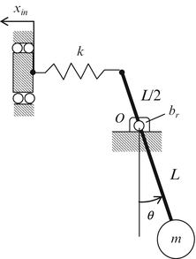
• 1. A positioning system is designed with a lever arrangement as shown in the figure. It is controlled by a displacement, x _in , applied through a spring. There is rotational viscous damping, b _r , in the pivot bearing at O.

  

  Complete the following.

  • (a) Determine the equation of motion for the system in terms of θ and linearize using the small angle approximation.

  • (b) Find the system transfer function $\frac{\Theta (s)}{X_{in}(s)}$.

  • (c) Determine the expression for the reflected rotational stiffness of the spring, k, and the reflected inertia of the mass, m.

  • (d) Determine expressions for the natural frequency, ω _n , and damping ratio, ζ.

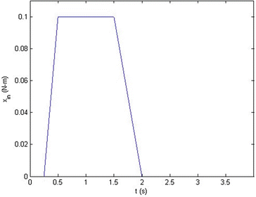
  • (e) The values of L, m, k, and b _r are 1.5 m, 2 kg, 500 N/m, and 10 N-m-s respectively. Calculate the natural frequency ω _n and damping ratio ζ. Using a Matlab ^® script file and the lsim command, simulate the response to the input provided and plot the response. The ramp up begins at 0.25 s and ends at 0.5 s. The ramp down begins at 1.5 s and ends at 2.0 s. The total time interval is 4.0 s.

    

  • (f) Repeat your simulation for a rotational damping, b _r , of 50 N-m-s. What is the new damping ratio? What is the effect on the response?

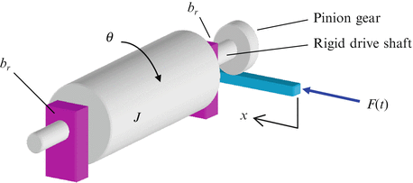
• 2. A rack and pinion drives system for a cylindrical drum in a chemical mixing system is depicted in the figure. The input is the force, F(t), which produces the motion, x, and rotates the pinion gear. There is viscous rotational damping, b _r , in each of the two bearings and the rotating drum has an inertia, J. The radius of the pinion gear is R and the shaft connecting the pinion to the drum is rigid.

  

  Complete the following.

  • (a) Determine the equation of motion in terms of v and $\dot{v}$, where $v=\dot{x}$.

  • (b) Determine expressions for the reflected inertia of the drum and the reflected damping of the bearings.

  • (c) Determine the equation of motion in terms of ω and $\dot{\omega}$, where $\omega =\dot{\theta}$.

  • (d) Find the transfer function $\frac{\Omega (s)}{F(s)}$ and the time constant for the system.

  • (e) The values of J, R, and b _r are 2.5 kg-m², 0.1 m, and 5 N-m-s, respectively. Using a Matlab ^® script file and the step command, simulate and plot the response ω(t) to an input force F(t) = F ₀ ⋅ u(t), where F ₀ is 500 N for a time interval of four time constants. Apply the final value theorem and initial value theorem to the solution in the Laplace domain and compare the results to your plot.

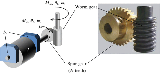
• 3. Consider the positioning system shown in the figure; it describes a rotary inertia, J, driven by a worm gear with an input moment, M _in (t). The worm gear drives a spur gear with N teeth so that ${\theta}_2=\frac{\theta_1}{N}$. The total rotational damping of the bearings is b _r and the shafts can be assumed to be rigid.

  

  Complete the following.

  • (a) Determine the equation of motion in terms of ω ₁ and ${\dot{\omega}}_1$.

  • (b) Determine and find expressions for the reflected inertia of J and the reflected damping of b _r at the worm gear input.

  • (c) Calculate the transfer functions $\frac{\Omega_1(s)}{M_{in}(s)}$ and $\frac{\Omega_2(s)}{M_{in}(s)}$ and determine an expression for the system time constant.

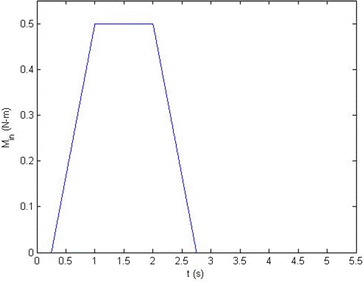
  • (d) The values of J, N, and b _r are 1.2 kg-m², 100 teeth, and 5 N-m-s, respectively. Using a Matlab ^® script file and the lsim command, simulate and plot the response ω ₂(t) to the input moment provided. The initial ramp up begins at 0.25 s and ends at 1.0 s. The ramp down begins at 2.0 s and ends at 2.75 s. The total time interval is 5.5 s.

    

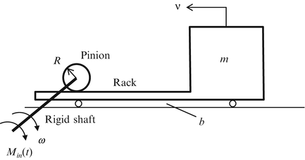
• 4. A motor on high-speed gantry machine tool drives a large mass with a moment, M _in (t), applied through a rack and pinion. The pinion radius is R and the mass is m. There is linear damping, b, acting against the motion of the mass from the oil slideways (linear bearings).

  

  Complete the following.

  • (a) Write the equations of motion in terms of, first, ω and M _in (t) and then v and M _in (t). Using the first equation, find an expression for the equivalent rotational inertia of the mass, m, as seen by the motor.

  • (b) The values of the parameters m, b, and R are 2000 kg, 400 N-s/m, and 0.2 m, respectively. The input moment is a step M _in (t) = M ₀ ⋅ u(t), where M ₀ is 10 N-m. Find the steady state velocity and time constant for the system.

  • (c) Find the velocity v(t) by solving the equation of motion using Laplace transforms.

  • (d) Use a Matlab ^® script file to plot the system response, v(t), to the step input for a duration of four time constants.

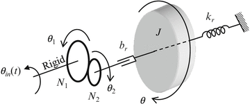
• 5. A disk with inertia, J, is attached to ground through a flexible shaft with rotational stiffness, k _r . It is driven through a fluid coupling with resistance (rotational damping), b _r , that connects gear 2 with N ₂ teeth to the inertia J. Gear 2 is driven by gear 1 with N ₁ teeth. The input is a prescribed angular displacement, θ _in (t), of gear 1 and the output is the angle θ(t) of the disk.

  

  Complete the following.

  • (a) Determine the equation of motion for the system in terms of θ and θ _in (t).

  • (b) The values of the parameters J and k _r are 0.05 kg-m² and 9000 N-m/rad, respectively. The gear ratio is 20:1 (N ₁ = 200 and N ₂ = 10). Calculate the natural frequency, ω _n , and determine the value of b _r such that the system is 40% damped.

  • (c) Using a Matlab ^® script file and the ilaplace command, find θ(t) in response to a ramp input θ _in (t) = 2t rad and plot the response for eight time constants. Apply the initial value theorem and final value theorem to the solution in the Laplace domain. Why does θ(t) reach a nonzero steady state value?