
Abstract
The identification of meaningful groups of proteins has always been a major area of interest for structural and functional genomics. Successful protein clustering can lead to significant insight, assisting in both tracing the evolutionary history of the respective molecules as well as in identifying potential functions and interactions of novel sequences. Here we propose a clustering algorithm for same-length sequences, which allows the construction of subset hierarchy and facilitates the identification of the underlying patterns for any given subset. The proposed method utilizes the metrics of sequence identity and amino-acid similarity simultaneously as direct measures. The algorithm was applied on a real-world dataset consisting of clonotypic immunoglobulin (IG) sequences from Chronic lymphocytic leukemia (CLL) patients, showing promising results.
You have full access to this open access chapter, Download conference paper PDF
Keywords
1 Introduction
One of the main challenges in computational biology concerns the extraction of useful information from biological data. This requires the development of tools and methods that are capable of uncovering trends, identifying patterns, forming models, and obtaining predictions of the system [1]. The majority of such tools and methods exist within the field of data mining. Clustering [2] is a data mining task that divides data into several groups using similarity measures, such that the objects within a cluster are highly similar to each other and dissimilar to the objects belonging to other clusters based on that metric. From a machine learning perspective, the search for meaningful clusters is defined as unsupervised learning due to the lack of prior knowledge on the number of clusters and their labels. However, clustering is a widely used exploratory tool for analyzing large datasets and has been applied extensively in numerous biological, genomics, proteomics, and various other omics methodologies [3]. Genomics is one of the most important domains in bioinformatics, whereas the number of sequences available is increasing exponentially [1]. Often the first step in sequence analysis, clustering can help organize sequences into homologous and functionally similar groups, can improve the speed of data processing and analysis, and can assist the prediction process.
There have been several approaches in the past, attempting to address the issue of identifying meaningful groupings of sequences of identical lengths. While sequence clustering has a long history in the field of bioinformatics ([4, 5]), there are few attempts in literature that can be successfully applied to sequences of the same length. One of the most notable approaches is the Teiresias algorithm [6, 7], that discovers rigid patterns (motifs) in biological sequences based on the observation that if a pattern spans many positions and appears exactly k times in the input, then all fragments (sub patterns) of the pattern have to appear at least k times in the input. The main drawback of this algorithm is that pairwise comparisons are employed between all the sequences of the dataset, leading to an exponential increase in execution time and memory requirements for large-scale datasets.
In this paper, we introduce a method for clustering amino acid sequences of identical length, using an approach that does not demand pairwise comparisons between the sequences, but it is instead based on the usage of a matrix that contains the amino acid frequencies for each position of the target sequences.
2 Methodology
The proposed clustering method uses both sequence identity and amino-acid similarity as similarity measures to form the clusters (both concepts are further defined below). Ultimately, a binary top-down tree is constructed by consecutively dividing the frequency amino acid matrix of a given cluster into two sub-matrices, until only two sequences remain at each cluster at the leaf-level.
2.1 Binary Tree Construction
The first phase consists of a top down hierarchical clustering method. Hierarchical clustering is one of the most commonly used approaches for sequence clustering [8]. At the beginning of the process, it is assumed that all Ν sequences belong to a single cluster, which is consequently split recursively while moving along the different levels of the tree. Ultimately, the constructed output of the clustering process is presented as a binary tree. The right side of the tree is expected to be much longer than the left side due to the constraints posed by the split process; the sequences with the highest similarity percentage at a specific sequence position are assigned to the right side, whereas the remaining sequences are assigned to the left. The process of this phase (Algorithm 1, Fig. 2) can be formally described in the following steps and further detailed below:
-
1.
Create frequency and frequency-similarity based matrix (FM, FSM)
-
2.
Compute average identity of the matrices (\( \overline{id} \), \( \overline{idS} \))
-
3.
Split each frequency matrix into two sub matrices
-
4.
Update the Level matrix and the Identity matrices (Y, I, IS)
-
5.
Check for branch break.
Step 1: Frequency amino acid and frequency-similarity based amino acid matrix.
The first aims to construct a frequency amino acid matrix. This is defined as a 2-dimensional matrix, with number of rows equal to the number of the different amino acids (i.e. 20 rows) and number of columns equal to the length (L) of the sequences provided as input. Each element (i,j) of the matrix corresponds to the number of times amino acid i is present in position j for all sequences. The count matrix (CM) contains the absolute values, whereas the frequency matrix (FM) contains the corresponding frequencies (Eq. 1). In addition to CM, a second frequency matrix is constructed using the same approach, but instead of the 20 amino acids, groups of similar amino acids are used under given schemes. As a use case in this paper, the 11 IMGT physicochemical classes are taken into consideration, as shown in Fig. 1, and an 11 x L frequency matrix is constructed.

The 11 IMGT Physicochemical classes for the 20 amino acids [9]. (Color figure online)

Block diagram of the tree construction.
Step 2: Compute Identity.
The identity is a similarity metric that is computed for each cluster based on the corresponding amino-acid frequency matrix. This metric, calculated as a percentage, indicates how compact the cluster is. Its maximum value (100%) corresponds to the case when the number of unique sequences that belong to a cluster is equal to one. The overall identity is equal to the average identity of each position in the given sequence (Eq. 2), and it is produced based on the CThr matrix, that contains only the elements of the amino acid matrix (CM) that correspond to amino acids that appear more than once in the corresponding column (Eq. 3).
Steps 3–4: Split of Frequency Matrices.
Each cluster is divided into two distinct subsets according to the following criteria and in the order that they are listed:
-
1.
Select the element of the frequency amino acid matrix with the highest percentage. An example of the division of cluster0 using this criterion is shown in Fig. 3.
Fig. 3. 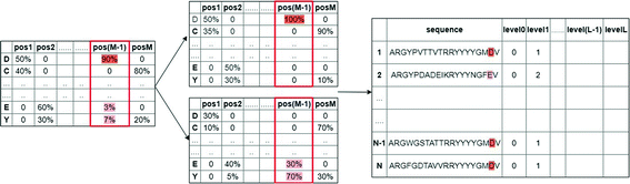
The division of Cluster 0 using the first criterion.
-
2.
If there exist more than one columns of the frequency amino acid matrix that contain the same highest percentage value, the selection is applied using the entropy criterion, defined below.
-
3.
In the case where more than one columns exhibit the exact same entropy value, criterion 1 is applied to the frequency similarity amino acid matrix.
-
4.
In the case of non-unique columns, criterion 2 is applied to the frequency similarity amino acid matrix.
-
5.
If the number of columns is still more than one, one column from the above sub group of columns is randomly selected.

Entropy criterion.
The entropy is computed for each column of the frequency matrix and represents the diversity of the column. A lower entropy value indicates a more homogeneous column, therefore the column with the lowest entropy value is selected during the splitting process.
Step 5: Branch Breaking.
Acluster is no further divided into subsets when the number of sequences that belong to the cluster is less than 3.
2.2 Software Implementation
The algorithm outlined in the paper is implemented in R, a programming language that is widely used for statistical computing, graphics and data analytics. In order to produce an interactive and user-friendly tool, thus making it easier for users to interact with the data, the analysis, and the visualization of the results, an R Shiny application was built using the shiny package. In practical terms, a Shiny App is a web page/ UI connected to a computer running a live R session (Server). The users can select personalized parameters via the UI. These parameters are passed on to the Server, where the actual calculations are performed and the UI’s display is updated according to the produced results.
R Shiny applications consist of at least two R scripts; the first one implements the User Interface ( ui.R ) by controlling the layout of the page using html commands and other nested R functions, and handles the input parameters provided by the users. The second script implements the Server ( server.R ) and contains essential commands and instructions on how to build the application and process the data. Except from those two essential scripts, a helper script is defined ( helpers.R ), which includes all the functions needed for further processing of the data and achieving the desirable plot formats.
Apart from the shiny package, several other packages have been utilized in order to add further functionality to the application and visualize the produced results. Indicatively, the DiagrammeR , data.tree and collapsibleTree libraries were very useful towards the visualization of the constructed tree. The latter is more interactive and gives the user the opportunity of collapsing branches and focusing on the branch or level of interest. Another special graph of our application is the logo graph, which contains the common letters of a specific cluster or level and can be produced through the use of the ggseqlogo library. Finally, our R Shiny Application is publicly available from the following URL:
https://github.com/mariakotouza/H-CDR3-Clustering.

3 Results
Our method was applied on a real-world dataset comprising 123 clonotypic immunoglobulin (IG) amino acid sequences (deduced from the corresponding IG gene rearrangement sequences) from patients with chronic lymphocytic leukemia (CLL). All sequences utilized the IGHV4-34 gene with 111 (90.2%) being assigned to 6 distinct biologically relevant groups (subsets), and had an identical length of 20 amino acids. These subsets are characterized by the presence of common amino acid sequence patterns within the VH CDR3 of the clonotypic IG. Subset #4 is a major subset and patients belonging to this subset display an indolent clinical course, while the other subsets are minor. In detail, 101 sequences were assigned to subset #4, 2 to subset #207, 2 to subset #4-34/20-1, 4 to subset #4-34-16, 2 to subset #4-34-18 whereas 12 sequences carried heterogeneous receptors and, thus, were not assigned to any subset.
Through the application of our tool, a binary tree with 19 levels was constructed (Fig. 5). The average value and the standard deviation of each level’s identity using the 20 amino-acid and the 11 IMGT Physicochemical classes are summarized in Table 1. The table shows that the identity value increased towards the leaves of the tree. Notably, when the 11 classes were used instead of the individual amino-acids, the total identity value was a little higher as expected.
In more detail, both Average Identity and Average Similarity values are equal to zero at the root of the tree and they almost consistently increase at each level, reaching the value of 98 percent on level 19. At any given point, the Average Similarity value is equal or greater than the Average Identity value, which is reasonable assuming that every similarity group contains one or more individual letters. Regarding the Identity Standard Deviation and Similarity Standard Deviation, it can be observed that both have an initial value of NA at the root, they are slightly increased for levels 1 and 2 and then their values decrease for every level until reaching the leaves. This is an expected outcome of the process, since the standard deviation is a measure of how spread out numbers are. Finally, the Identity Standard Deviation is equal to or greater than Similarity Standard Deviation, because the number of individual letters is greater than the number of similarity groups and therefore the amount of spread is higher.
Figure 4 shows the logos of four clusters from four different levels of the tree. The size of each amino-acid indicates the percentage of its occurrence at the specific position of the CDR3 sequence, whereas the color of the amino-acid represents the IMGT Physicochemical class it belongs to. The color code used for the logo figures is consistent with the color scheme shown in Fig. 1.

CDR3 region logos of four clusters of different levels of the tree.
Subset #4 is the largest subset in the present data series comprising 101 clonotypic IG sequences. Most of them (93/101, 92%) formed cluster 13, at level 4 of the clustering process, with level 0 being the root of the tree. Cluster 13 also included 3 non-subset IG sequences. The identity and similarity rates of this cluster were 20% and 30%, respectively. The CDR3 of cluster 13 is 20 amino acids long and consisted of 4 conserved positions and 16 positions that are characterized by variability. Subset #4-34/20-1 consisted of 2 clonotypic IG sequences. These sequences were grouped together at level 9 (cluster 57) with high identity and similarity rates (80% and 95%, respectively). Only 4 positions of the CDR3 were encoded by different amino acids: A R Y _ _ V V T A _ _ N Y Y Y Y G M D V . More uniform groups and less variability at a position level is noticed at higher levels of clustering. Consequently, identity and similarity rates increase from one level to another. Subset #4-34-16 consisted of 4 clonotypic IG sequences. Three out of 4 IG sequences (75%) were grouped together at level 5 forming cluster 31 with 45% identity and 50% similarity. Cluster 31 also included a non-subset IG sequence. At the next level of clustering (level 6) the sequences assigned to subset #4-34-16 (3/4, 75%) formed cluster 39 with higher identity and similarity rates (70%|80%). Six positions were characterized by variability.

The binary tree with 12 levels and values for each cluster with the format [cluster id, number of cluster sequences, identity, similarity]
4 Discussion
In this study, we applied a new clustering technique to 123 immunoglobulin (IG) sequences of the CDR3 region from patients with chronic lymphocytic leukemia (CLL), all of which express the IGHV4-34 gene. This is a hierarchical method that constructs a top-down binary tree by iteratively breaking the amino-acid frequency matrix into two sub-matrices and using identity and amino-acid similarity as measures for the clustering. The results of this analysis showed that the identity value increases as one transitions from the root towards the leaves of the tree. In the case when the 11 IMGT Physicochemical classes were used instead of the 20 individual amino-acids, the identity value was a little higher as expected.
The proposed method can extract patterns from the clusters at the different tree levels. For example, the pattern that corresponds to cluster 13 (as shown in Fig. 4a) is _ R _ _ _ _ _ _ _ _ _ _ Y _ Y _ G _ _ _, whereas the consensus pattern of cluster 39 (Fig. 4d) is _ _ _ V V P A A _ _ P _ Y Y Y Y G M D V . These patterns can be directly used by biomedical experts in order to evaluate the cluster and infer potential meaningful interaction at the amino acid level. In our case, clustering is performed to discover previously unknown patterns (unsupervised learning) and then, as a next step, sequence labeling can be performed to assign new sequences to the existing classes.
Future steps involve the application of graph theory on the produced tree, in conjunction with string distance metrics, in order to further refine the clustering process and uncover potential connections between different clusters/ nodes of the tree. Moreover, additional testing will be required, especially focusing on large-scale datasets and optimizing the code for speed and memory usage.
References
Pedro Larranaga, R.S., Robles, V.: Machine learning in bioinformatics. Brief. Bioinform. 7, 86–112 (2006)
Berkhin, P.: A survey of clustering data mining techniques. In: Kogan, J., Nicholas, C., Teboulle, M. (eds.) Grouping Multidimensional Data, pp. 25–71. Springer, Berlin (2006). https://doi.org/10.1007/3-540-28349-8_2
Belacel, N., Cuperlovic-Culf, M.: Clustering: Unsupervised Learning In Large Screening Biological Data (2010)
Li, W., Godzik, A.: Cd-hit: a fast program for clustering and comparing large sets of protein or nucleotide sequences. Bioinformatics 22(13), 1658–1659 (2006)
Edgar, R.C.: Search and clustering orders of magnitude faster than BLAST. Bioinformatics 26(19), 2460–2461 (2010)
Rigoutsos, I., Floartos, A.: Combinatorial pattern discovery in biological sequences: The TEIRESIAS algorithm. Bioinformatics (Oxford, England), 14, 55–67 (1998)
Darzentas, N., Hadzidimitriou, A., Murray, F., Hatzi, K., Josefsson, P., Laoutaris, N., Moreno, C., Anagnostopoulos, A., Jurlander, J., Tsaftaris, A., Chiorazzi, N., Belessi, C., Ghia, P., Rosenquist, R., Davi, F., Stamatopoulos, K.: A different ontogenesis for chronic lymphocytic leukemia cases carrying stereotyped antigen receptors: molecular and computational evidence. Leukemia 24, 125–132 (2010)
Cai, Y., Zheng, W., Yao, J., Yang, Y., Mai, V., Mao, Q., Sun, Y.: ESPRIT-forest: parallel clustering of massive amplicon sequence data in subquadratic time. PLoS Comput. Biol. 13, e1005518 (2017)
IMGT, The International ImMunoGeneTics Information System. (http://www.imgt.org)
Acknowledgments
The authors would like to thank Katerina Gemenetzi, Andreas Agathangelidis and Kostas Stamatopoulos from the Institute of Applied Biosciences (INAB|CERTH) for providing the dataset as well as for their critical review of the paper.
Author information
Authors and Affiliations
Corresponding author
Editor information
Editors and Affiliations
Rights and permissions
Copyright information
© 2018 IFIP International Federation for Information Processing
About this paper

Cite this paper
Tsarouchis, S., Kotouza, M.T., Psomopoulos, F.E., Mitkas, P.A. (2018). A Multi-metric Algorithm for Hierarchical Clustering of Same-Length Protein Sequences. In: Iliadis, L., Maglogiannis, I., Plagianakos, V. (eds) Artificial Intelligence Applications and Innovations. AIAI 2018. IFIP Advances in Information and Communication Technology, vol 520. Springer, Cham. https://doi.org/10.1007/978-3-319-92016-0_18
Download citation
DOI: https://doi.org/10.1007/978-3-319-92016-0_18
Published:
Publisher Name: Springer, Cham
Print ISBN: 978-3-319-92015-3
Online ISBN: 978-3-319-92016-0
eBook Packages: Computer ScienceComputer Science (R0)